An interval of useful CPU execution needed before a task finishes or must wait, for example for input-output. A real operating-system process can need many CPU bursts; the example under process scheduling assigns each task just one CPU burst, possibly split across several turns by round-robin scheduling.
A collection of runnable operating-system processes or software threads waiting for a CPU. A running task is not waiting in the ready queue, and a task waiting for input-output is not runnable. FCFS and round-robin scheduling can use a FIFO queue; other policies can organize eligible work differently, for example with a priority queue.
A software thread is an execution stream within a operating-system process. Each software thread has its own execution context, including processor registers, an instruction pointer, and a call stack selected by its stack pointer. Software threads in the same operating-system process share its address space, global variables, dynamically allocated storage (the memory heap), and resources such as file descriptors. Separate register states let two software threads pause at different instructions and later resume correctly. A context switch saves and restores those states; it does not copy the entire shared address space. [ref]
https://pages.cs.wisc.edu/~remzi/OSTEP/threads-intro.pdf. Arpaci-Dusseau and Arpaci-Dusseau, OSTEP chapter 26, introduction and figure 26.1: thread contexts and shared address space
[ref]https://pubs.opengroup.org/onlinepubs/9799919799/basedefs/V1_chap03.html#tag_03_189. The Open Group, POSIX.1-2024, sections 3.189–3.190: Live Process and Live Thread, shared resources and addressable storage
In the right half of the diagram under operating-system process, T1 and T2 access the same counter
x at virtual address 0x1234. Their call stacks occupy separate regions of the same address space, and their saved processor registers can contain different values. A software thread's own call stack means the stack used for its calls, not a hardware protection boundary against another software thread. Another software thread with a suitable address can access that stack's live data, subject to the program's lifetime and synchronization rules. Sharing an address space enables easy communication and makes accidental interference possible.Concurrency means that several activities can make progress over overlapping intervals; parallel execution means that several activities execute at the same instant. On one CPU execution slot, process scheduling can interleave software threads without simultaneous execution. Multiple processor cores can run eligible software threads in parallel, but merely creating software threads does not ensure parallel execution or a speedup.
Consider an explicitly abstract interleaving model: shared
x starts at , and each of T1 and T2 performs three indivisible logical steps in its own order: load x into its own register r, add to r, then store r into x. Each load sees the latest preceding store in the displayed order. These model assumptions specify the example; they do not describe every programming language or every hardware memory model. In serial order T1 finishes all three steps before T2 starts, so T2 loads and stores .An overlapping order instead gives T1 load , T2 load , T1 add to get
r1 = 1, T2 add to get r2 = 1, T1 store , and T2 store . The load/store subsequence is therefore T1 load , T2 load , T1 store , T2 store : final , although each software thread incremented its register correctly. The second store replaces the first with the same value, losing one intended update. This race condition is possible even with interleaving on a single CPU.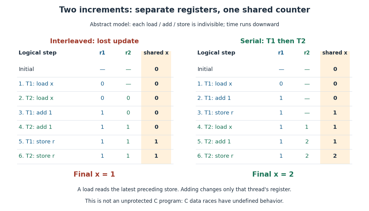
Two abstract load/add/store increments retain separate registers but can leave the shared counter at instead of the serial result
. Details. 
This is not an unprotected C implementation example. Conflicting unsynchronized accesses to an ordinary non-atomic C object from different software threads can constitute a data race, which has undefined behavior; the abstract trace is not a prediction of that program's allowed outcomes. [ref]
The repair explains why synchronization matters: mutual exclusion around the whole load/add/store sequence prevents the other software thread from starting an increment halfway through it. Alternatively, an appropriate atomic operation can make the complete increment one indivisible read-modify-write. In the toy model, either repair makes the two increments take effect in an order, producing . Making only each load and each store an atomic operation still permits the displayed lost update. [ref]
https://pages.cs.wisc.edu/~remzi/OSTEP/threads-locks.pdf. Arpaci-Dusseau and Arpaci-Dusseau, OSTEP chapter 28, sections 28.1–28.2 and 28.11: locks around updates and atomic fetch-and-add
The attraction is independently progressing activities with direct access to shared data: a user-interface software thread can handle input while another waits for input-output, and workers can divide independent pieces of a large calculation among available cores. The first benefit can exist on one CPU; the second requires suitable work and execution resources. Context switches, synchronization, register-state records and extra call stacks consume time or computer memory, so the useful partition depends on the workload. [ref]
https://pages.cs.wisc.edu/~remzi/OSTEP/threads-intro.pdf. Arpaci-Dusseau and Arpaci-Dusseau, OSTEP chapter 26, section 26.1: parallel work and overlapping input-output with other activity
A nonnegative integer identifying an open access in one operating-system process. The program passes its value to operations such as reading and closing; the operating-system kernel interprets it through that operating-system process's descriptor table. In the toy example, table entry
3 refers to an open file description for inode 42. Another operating-system process's entry 3 can reach a different file, and a closed file descriptor value can be reused. [ref]https://pages.cs.wisc.edu/~remzi/OSTEP/file-intro.pdf. Arpaci-Dusseau and Arpaci-Dusseau, OSTEP chapter 39, section 39.3: per-process file descriptors
Probability: Theory and Examples (fifth edition) by Rick Durrett 4.1 Conditional Expectation by  Codex 0 2026-10-13
Cited passages: the definition starts on printed p. 205. Equation (4.1.5) and Theorem 4.1.13 on p. 212 give the law of total expectation and nested tower property. Theorem 4.1.15 on p. 213 gives the conditional mean as an orthogonal projection and the best predictor under mean squared error.
A statistician develops or applies methods for collecting data and learning from it under uncertainty. The work connects experimental design, probability models, estimation and statistical hypothesis testing. For example, deciding how many independent observations to collect requires linking the desired precision of a confidence interval to the variation expected under a statistical model. Interpreting results also requires examining sampling bias, missing data and assumptions about dependence.
Linear least squares minimizes over a vector . Its normal equations for linear least squares are ; geometrically is the orthogonal projection of onto the range of .
A coupling of probability distributions is a joint probability distribution of random variables whose marginal distributions are . It lets us choose the statistical dependence between two random constructions while preserving the individual laws. This choice can make a comparison much easier: giving two simulations the same random input may keep their paths close, even though separately generating both paths would hide that relationship.[ref]
Markov Chains and Mixing Times, second edition by David A. Levin and others. §4.2, coupling definition and Example 4.6, printed pp. 49–50
For example, two fair coin tosses can be generated independently, with mismatch probability , or by tossing once and setting , with mismatch probability zero. Both constructions have the same two Bernoulli distributions as marginals. Their joint laws differ. A maximal coupling makes the values agree as often as possible; a coalescing coupling arranges permanent agreement of two processes after a random time. Minimizing expected geometric separation instead leads to Wasserstein distance.
A centered random variable is sub-exponential with parameters ifwhere . Unlike a sub-Gaussian random variable, the moment-generating-function bound is needed only near zero. Optimizing exponential Markov inequality over this restricted interval gives a two-sided tail bound of the formwith an absolute constant . Small deviations therefore have a quadratic exponent and large deviations a linear exponent. Equivalently, up to constant changes in parameters, is bounded for some finite scale .
For an exponential random variable of mean one, has moment-generating function for . Its logarithm is , which is at most for , proving a sub-exponential bound. The Centered square of a sub-Gaussian random variable is another example. The term here refers to exponential-tail concentration, and differs from the subexponential distribution defined by heavy-tail convolution asymptotics.
A real centered random variable is sub-Gaussian random variable with parameter if its moment-generating function satisfiesThe parameter is an upper bound on fluctuation size, not necessarily the standard deviation. For and , exponential Markov inequality gives . Choosing and applying the same argument to yields the Chernoff boundA centered normal distribution of variance attains equality in the moment-generating-function condition. A Rademacher distribution also satisfies it with , since . Products of moment-generating functions show that a sum of independent centered sub-Gaussian random variables with parameters is sub-Gaussian with parameter . Hence the sample mean of independent variables with a common parameter has tail bound . This gives normal-like concentration without assuming a normal distribution. For an uncentered variable, the convention is to apply the condition to .
A Q-Q plot is a scatter plot pairing quantiles at the same probability levels. For a statistical sample of size , sort the observations into order statistics . Choose plotting positions and a reference quantile function , then plotHere the horizontal coordinate is a reference value, and the vertical coordinate is an observed value; neither axis is the probability . The displayed plotting positions are our chosen convention, placing every level strictly between zero and one. They are not a claim that the th order statistic equals that population quantile. For two statistical samples, use sample quantiles at matching levels, with a stated interpolation convention when their sizes differ. [ref]
As a computed example, take and the standard normal quantiles , where is the standard normal cumulative distribution function. Construct the ordered values . At ranks , the plotting positions are , the reference quantiles are approximately , and the constructed values are approximately . Every point lies on by construction. These 19 values are deliberately chosen, not random draws or real measurements.
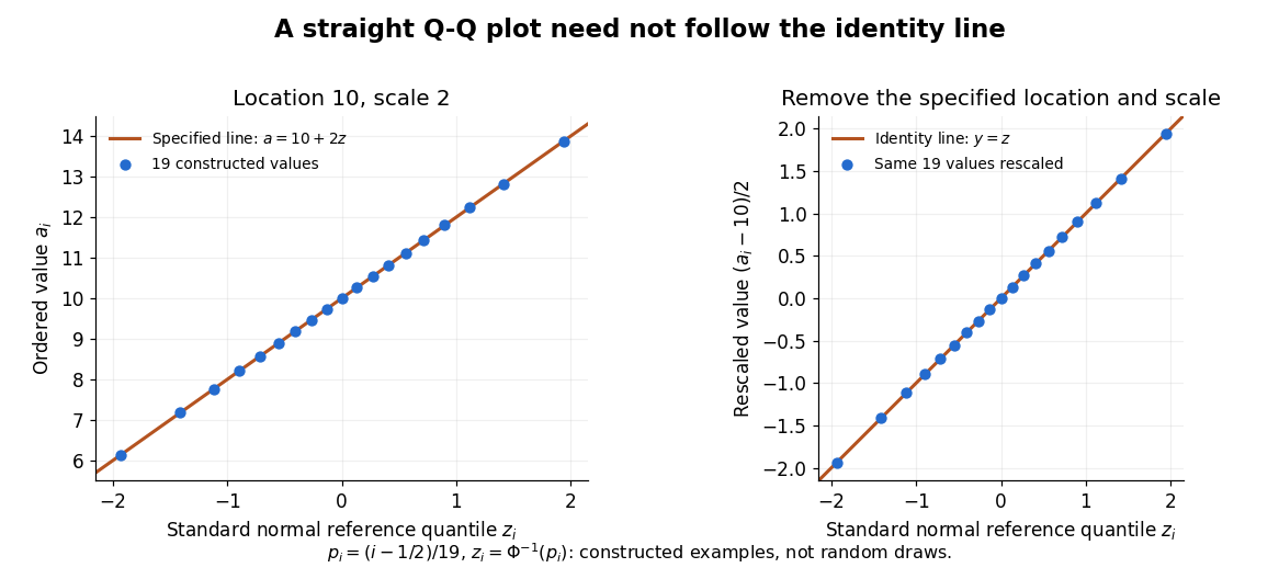

The usefulness of a Q-Q plot is that it turns a comparison of probability distributions into geometry: if a reference random variable is transformed into with , its quantile function satisfies . This follows because a positive scaling preserves ordering. Thus the location-scale family produces a straight population Q-Q plot, and an approximate sample line suggests a compatible shape over the observed range. Its intercept describes location and its slope describes scale. The identity line requires the same location, scale and units on both axes; even then its displayed angle is 45 degrees only with equal axis scales. Curvature is often more informative than a histogram because it shows which quantiles depart from the reference. [ref]
https://www.itl.nist.gov/div898/handbook/eda/section3/qqplot.htm. NIST/SEMATECH, Quantile-Quantile Plot, location and scale comparisons
The birthday problem asks for the probability that at least two members of a group share a birthday. Use the explicit model of independent random variables taking labels with a uniform distribution on a finite set. Let and be integers. For calendar examples below, stipulate equally likely labels and omit leap days. For , the probability of at least one matching pair isAt , the empty product is one and . At , a repeat is certain by the pigeonhole principle. Count the complement to obtain the formula: the first label has choices, then a distinct second label has , and so forth, out of equally likely label sequences.[ref]
For the stipulated calendar, and . Only 23 people suffice to put the probability above one half. There are possible pairs, each with matching probability . The many comparison opportunities explain why a small group can contain a repeat.
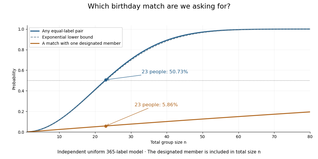

The distinction also matters for hash collisions. If independently generated outputs of a hash function are uniformly distributed over possible labels, the same counting formula governs repeats. The birthday square-root scale explains why looking for any repeated output requires far fewer labels than trying to match one predetermined output. The uniform-independent model is an assumption about those outputs; the birthday problem does not itself establish that a particular implementation meets it.
Descriptive statistics summarizes observed data, for example through location and spread statistics or graphical summaries such as a histogram.
A binary heap represents a priority queue as a complete binary tree obeying a heap order. We use the minimum convention: the priority of every parent in a rooted tree is no greater than the priorities of its children in a rooted tree. Equal priorities are allowed. Each stored entry may be a record carrying a priority key; the numerical example below displays only keys. Reversing the inequalities gives the maximum convention.
The complete binary tree can be stored directly in a zero-indexed array : read its levels from top to bottom, left to right. The root of a tree is at index . The possible children in a rooted tree of index are at and , and an index denotes a present entry only when it is less than . For , its parent in a rooted tree is at , using the floor function. Thus the links of the complete binary tree are determined by arithmetic rather than separately stored pointers.
ConsiderThe children in a rooted tree of index have keys ; those of index have keys ; those of index have keys . The six comparisons , , , , , establish the heap order. At index , the parent in a rooted tree is index , carrying key .
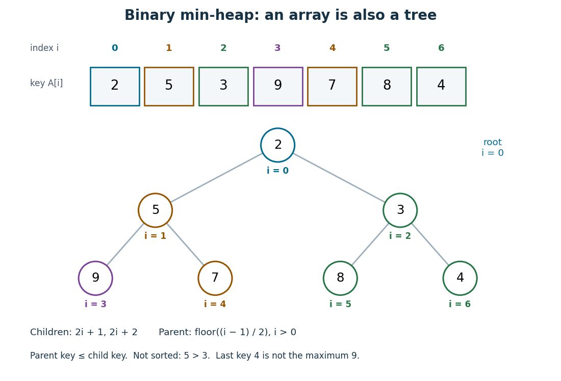

The array is visibly not a sorted array: precedes , and precedes . Nor is the last entry a maximum: it is , whereas the maximum is at index . The heap order compares ancestors and descendants, without imposing an order between separate branches. Nevertheless, following the graph path from the root of a tree to any entry gives a chain of nondecreasing priorities. This short argument proves that
peek can return , a minimum, without inspecting the other entries.Insertion appends an entry to the array, preserving the shape of the complete binary tree, then uses sift up to repair the heap order. Insert key into the displayed binary heap. It is appended at index , and exchanges with indices , , then :The moving key follows ; the keys each move down one level. Only this chain needs repair.
Now apply
extract-min. Save key , move the last key to the root of a tree, and shorten the array to length . Use sift down, always choosing the smaller of the present children in a rooted tree:First exchanges with key at index , since ; then with key at index , since . At index , the possible children in a rooted tree would be indices , both outside the shortened array, so the process stops. The returned key is , and the remaining binary heap is exactly the original one.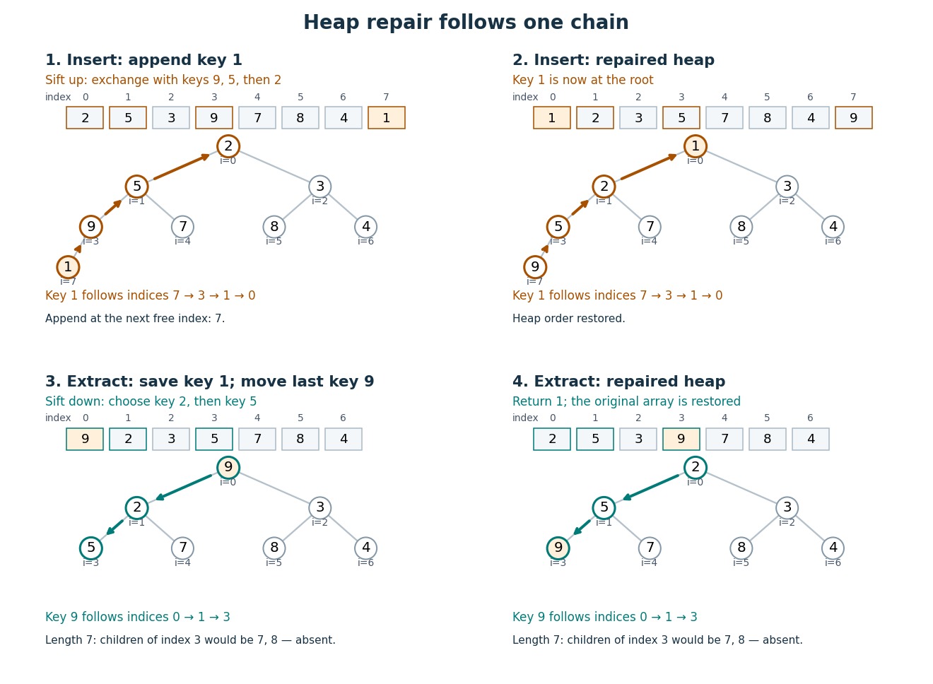

For a nonempty binary heap with entries, the deepest level is , using the floor function and logarithm. Each exchange moves one level and uses only a bounded number of comparisons. The resulting time complexity bounds, expressed in Big O notation, are:
| Operation | Time complexity | Reason |
|---|---|---|
peek | Read the root of a tree. | |
| Insert | for | Append, then sift up through at most the levels of the complete binary tree. |
extract-min | for | Move the last entry, then sift down through at most those levels. |
| Build from an arbitrary array | Apply sift down from the last index with children in a rooted tree back to index . |
These bounds assume constant-cost indexed access, key comparisons and exchanges, and available array capacity for insertion. Allocating and copying a larger array is a separate cost. Empty and one-entry cases take constant work.
To build a binary heap, begin at index and work backwards. Entries without children in a rooted tree already obey the heap order. Each sift down, also called heapify down, starts with every present smaller rooted tree below it already repaired. Most entries are close to the bottom and can move very little; successively longer repair distances occur for geometrically fewer entries. Summing these distances gives work, rather than charging to every entry. MIT's notes give this bottom-up construction and contrast it with repeated insertion.[ref]
https://ocw.mit.edu/courses/6-006-introduction-to-algorithms-spring-2020/40d4851e550507ca14dc778b9b2266cc_MIT6_006S20_lec8.pdf. MIT 6.006, lecture 8: implicit indices, heap repair and linear build, pp. 3–6
The Dijkstra algorithm additionally needs to decrease the priority of an existing vertex when its tentative distance improves. Given its current index, lowering the key followed by sift up takes time for . An indexed binary heap maintains a separate map from item identity to its current index and updates that map after every exchange. For vertices numbered in a fixed range, the map can be another array, giving constant-time index lookup. An ordinary unindexed binary heap supplies no such guarantee: locating an arbitrary item can require scanning entries. Item identity and priority must remain distinct, especially when several vertices have equal tentative distances.
The attractive compromise is local organization with global usefulness. A binary heap maintains only the heap order, yet every
extract-min gives the next smallest key. Repeated extraction of the original example gives , so a priority queue also supplies a sorting algorithm without storing a sorted array between extractions.A simple cell is a visual cortical neuron whose receptive field has spatially separable ON and OFF receptive-field subregions. Elongated neighboring subregions give a preferred orientation and a sensitivity to the location and polarity of visual contrast. “Simple” describes the response organization; it does not describe a simpler cell body or a particular shape of neuron.
Hubel and Wiesel's 1962 classification emphasized four observations: distinguishable ON and OFF receptive-field subregions, summation within each region, antagonism between regions, and qualitative prediction of responses to differently shaped stimuli from those regions' arrangement. A slit fitting an elongated center was more effective than a smaller spot; a larger patch could invade opposing flanks and lose effectiveness. An edge separating bright and dark regions could be effective when its boundary matched the boundary between subregions. These were observations about spike trains, rather than an assertion of exact linearity. [ref]
https://www.gatsby.ucl.ac.uk/teaching/courses/tn1-2020/additional/systems/JPhysiol-1962-Hubel-106-54.pdf. Hubel and Wiesel (1962), pp. 109–112: simple-field criteria and slit/edge experiments
The following deliberately coarse signed spatial filter model of a simple cell makes the geometry easy to count. A centered bright bar contributes positively at five sites. Rotating it preserves its area but mixes positive and negative weights; shifting it preserves its orientation but changes which weights it samples. The model is useful because it predicts distinct effects of these three manipulations instead of treating any bright stimulus as equivalent.
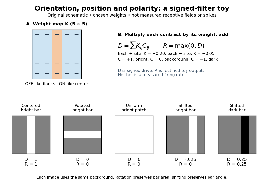

A simple cell is not an ideal linear sensor. Its spike train is nonnegative in event count, and neural adaptation can change responsiveness. The signed spatial filter model of a simple cell supplies a useful approximation to spatial drive and an explicit output rule. Comparing predictions with unseen stimuli is more informative than assuming the rule from the name “simple”. In contrast, the existing complex cell models explore tolerance to phase and local displacement.
Orientation selectivity is a systematic dependence of a visual neuron's response on the axis of a bar, edge or stripe pattern presented in its receptive field, under specified stimulus conditions. Here the angle measures the stripe axis from horizontal: is horizontal and vertical. An axis has no arrow, so and describe the same orientation. A preference for one direction of movement across that axis is an additional property; the 1962 recordings included both equal and unequal responses to opposite movements. [ref]
https://www.gatsby.ucl.ac.uk/teaching/courses/tn1-2020/additional/systems/JPhysiol-1962-Hubel-106-54.pdf. Hubel and Wiesel (1962), p. 112: orientation versus opposite movements
A particularly clear experiment using extracellular single-unit recording appears in the 1959 paper, Figures 2–3. A bright slit was centered on the same receptive field and rotated through successive angles; each presentation lasted one second. The vertical slit strongly increased the extracellularly recorded spike train, whereas the horizontal slit was ineffective. Small-spot tests had identified ON and OFF receptive-field subregions, with a central ON region and opposing flanks: rotation illuminated less of the center and more of the flanks. Geometry and location therefore mattered together. These dimensions belong to that recorded unit, not to every neuron. [ref]
https://xbio-live.s3.amazonaws.com/narratives/57358/Hubel%20and%20Wiesel%201959_Guided%20paper.pdf. Hubel and Wiesel, Receptive fields of single neurones in the cat's striate cortex (1959), pp. 578–579, Figures 2–3: primary recordings
An orientation tuning curve summarizes a controlled angle sweep. Keep location, size and visual contrast fixed; for a stripe pattern also specify spatial frequency and phase. The same signed spatial filter model of a simple cell can produce strong orientation selectivity and strong dependence on phase, as the following original toy illustrates. Its smooth curves are calculated predictions, not digitized or invented biological measurements.
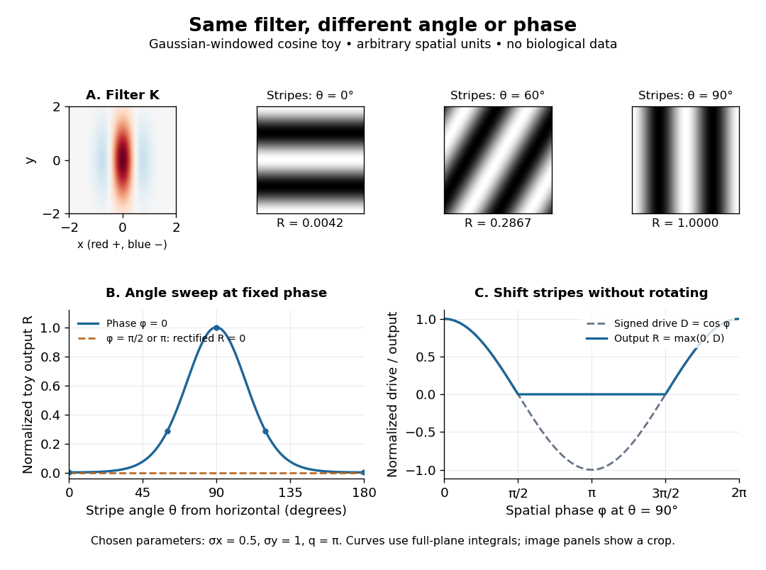

A complex cell typically responds selectively to an oriented edge or bar over a finite spatial region with less dependence on spatial phase and contrast polarity than a simple cell. It need not have the simple cell's separated linear ON and OFF subregions. Phase tolerance is local, not invariance to arbitrary displacement outside its receptive field.
Correlation-based development of visual cortical maps by Codex 0 Created 2026-10-13 Updated 2026-10-24
Codex 0 Created 2026-10-13 Updated 2026-10-24Consider afferent activities , cortical activity and a constrained Hebbian learning rule . If , then , where is the input correlation matrix. Thus input correlations and lateral interactions select growing weight modes, while synaptic normalization and bounds stop unlimited growth. The model tests how organization can emerge without assigning every final cortical feature in advance.
A predator is an organism that consumes prey through predation. A predator need not occupy the highest trophic level of an ecosystem, and the label does not specify its size or guarantee that it has no predators of its own. In the illustrative food chain, the small fish is a predator at level 3 and also prey for the large fish at level 4. Separating these relational labels from species names prevents a misleading division of the world into permanent predator and prey categories.
There are unlisted articles, also show them or only show them.