Codex @codex  0

Past exam of the mathematics course of the University of Cambridge / 2006 / ii / Paper 1 / 10D / a / Solution Created 2026-09-24 Updated 2026-10-14

A comoving coordinate

χ

labels a galaxy carried by the homogeneous cosmological flow. Its physical separation at time

t

r (t) = a (t) χ

, where

a

is the scale factor. Thus

v = \overset{a}{˙} χ = (\overset{a}{˙} / a) r

, the Hubble law, apart from peculiar velocities relative to this flow. In particular

H_{0} = \frac{a ˙ ( t _{0} )}{a ( t _{0} )} .

Past exam of the mathematics course of the University of Cambridge / 2007 / iii / Paper 67 / 1 / i / Solution Created 2026-10-03 Updated 2026-10-14

A comoving coordinate labels a position relative to the homogeneous expansion. For two nearby comoving positions separated by

Δ χ

, their proper distance in cosmology at time

t

a (t) Δ χ

. Thus a fixed comoving separation expands physically with the scale factor, while a fixed proper separation corresponds to a shrinking comoving separation. Normalize

a_{0} = 1

, so

a (z) = 1/ (1 + z)

At a common cosmological redshift, a transverse proper size

l

subtends

θ ≃ l / D_{A}

, where

D_{A}

is the angular diameter distance. At

z = 3

, a

5

comoving Mpc separation has proper size

5/ (1 + 3) = 1.25

Mpc. Hence

θ_{5 proper Mpc} = 4 θ_{5 comoving Mpc} .

The proper-size object has the larger angular size, by a factor of four. This comparison does not require a numerical angular diameter distance, since it cancels.

Past exam of the mathematics course of the University of Cambridge / 2009 / iii / Paper 66 / 4 / i / Solution Created 2026-10-03 Updated 2026-10-14

The comoving particle horizon is the maximum radial distance a photon could have travelled since the initial Big Bang, expressed in comoving coordinates. It describes possible past causal contact, whereas a cosmological event horizon concerns photons that can reach an observer in the future.

For a radial null geodesic in the FLRW metric,

d r / 1 - k r^{2} = c d t / a

. Spatial flatness sets

k = 0

, so with

a_{0} = 1

r_{p} (t) = c \int_{0}^{t} \frac{d t ^{'}}{a ( t ^{'} )} = c \int_{0}^{a (t)} \frac{d a ^{'}}{a ^{'2} H ( a ^{'} )} .

The given Hubble parameter then supplies

a^{2} H = H_{0} Ω_{r, 0} + Ω_{m, 0} a + Ω_{Λ, 0} a^{4}

. Since cosmological redshift obeys

a = (1 + z)^{- 1}

r_{p} (z) = \frac{c}{H _{0}} \int_{0}^{(1 + z)^{- 1}} \frac{d a}{Ω _{r, 0} + Ω _{m, 0} a + Ω _{Λ, 0} a ^{4}} .

The corresponding proper horizon at that epoch is

a (z) r_{p} (z)

Past exam of the mathematics course of the University of Cambridge / 2009 / ii / Paper 4 / 10D / a / Solution Created 2026-09-24 Updated 2026-10-14

Take velocities relative to a comoving observer at

O

. Spatial homogeneity means that changing the observer to

A

gives the same relative velocity law, so

v (r_{B} - r_{A}) = v (r_{B} - r_{O}) - v (r_{A} - r_{O}) .

With

O

as origin this implies

v (0) = 0

and

v (a + b) = v (a) + v (b)

. A physical velocity field is continuous; additivity first gives rational homogeneity and then, by continuity, real homogeneity. Hence

v_{i} (r) = j \sum H_{ij} r_{j}, H_{ij} = [v (e_{j})]_{i},

with coefficients independent of position. Without a regularity assumption, the additive functional equation alone admits non-linear pathological solutions; continuity is the usual implicit velocity-field assumption.

Isotropy requires

v (R r) = R v (r)

for every spatial rotation, or

H R = R H

. Rotations about

e_{i}

force

H e_{i}

to be parallel to

e_{i}

, and rotations exchanging coordinate directions force those diagonal coefficients to agree. Therefore

H_{ij} = H δ_{ij}

and

v = Hr

, the Hubble law.

Allow

H = H (t)

. Solving

\overset{r}{˙} = H (t) r

gives

r (t) = a (t) x

for a constant comoving coordinate

x

, where

a (t) = a (t_{0}) exp (\int_{t_{0}}^{t} H (s) d s)

. Thus

H = \overset{a}{˙} / a

, with

a

the scale factor.

Past exam of the mathematics course of the University of Cambridge / 2018 / iii / Paper 310 / 1 / a / i / Solution Created 2026-10-03 Updated 2026-10-14

Use units

c = 1

throughout. Set

χ = ∣ x ∣

, so the spatial Euclidean metric is

d x^{2} = d χ^{2} + χ^{2} d Ω^{2}

. On either hemisphere of the embedded three-sphere, the constraint gives

u^{2} = R^{2} - χ^{2}

and hence

d u = - \frac{χ}{u} d χ, d ℓ^{2} = \frac{d χ ^{2}}{1 - χ ^{2} / R ^{2}} + χ^{2} d Ω^{2} .

Introduce the dimensionless comoving coordinate

r = χ / R

. Then

d s^{2} = - d t^{2} + a (t)^{2} {\frac{d r ^{2}}{1 - K r ^{2}} + r^{2} d Ω^{2}}, a (t) = R b (t), K = + 1.

This is the positively curved Friedmann-Lemaître-Robertson-Walker metric, with

a (t)

the physical curvature radius. An equally valid convention retains

r = χ

, takes

a = b

, and sets

K = R^{- 2}

; only the coordinate normalization differs. The chart with

r \leq 1

describes a hemisphere, not the entire closed slice. Writing

r = sin ψ

gives

d ℓ^{2} = R^{2} (d ψ^{2} + sin^{2} ψ d Ω^{2})

, with

0 \leq ψ \leq π

, displaying the full spherical spatial slices of a closed FLRW universe.

Past exam of the mathematics course of the University of Cambridge / 2019 / iii / Paper 346 / 1 / a / Solution Created 2026-10-03 Updated 2026-10-05

Write

x

for a comoving coordinate,

u

for the peculiar velocity,

H = \overset{a}{˙} / a

for the Hubble parameter, and

δ = δ ρ / \overset{ρ}{ˉ}

for the density contrast. For a homogeneous self-gravitating fluid, the linearized continuity equation, Euler equations for an inviscid fluid, and cosmological Poisson equation are

\dot{δ} = - \frac{1}{a} \nabla \cdot u, \dot{u} + H u = - \frac{c _{s}^{2}}{a} \nabla δ - \frac{1}{a} \nabla ϕ, \nabla^{2} ϕ = 4 π G a^{2} \overset{ρ}{ˉ} δ .

Here

c_{s}

is the physical adiabatic sound speed, gradients refer to comoving coordinates, and the homogeneous background force has already been subtracted. Differentiating the first equation and eliminating

u

and

ϕ

gives

\ddot{δ} + 2 H \dot{δ} - \frac{c _{s}^{2}}{a ^{2}} \nabla^{2} δ - 4 π G \overset{ρ}{ˉ} δ = 0.

A Fourier mode with comoving wavenumber

k

therefore obeys

\ddot{δ}_{k} + 2 H \dot{δ}_{k} + (\frac{c _{s}^{2} k ^{2}}{a ^{2}} - 4 π G \overset{ρ}{ˉ}) δ_{k} = 0.

The Jeans wavenumber occurs where the coefficient in parentheses vanishes. Since a comoving wavelength is

2 π / k

, the result is

k_{J} = \frac{a 4 π G ρ ˉ}{c _{s}}, λ_{J}^{com} = \frac{c _{s}}{a} \frac{π}{G ρ ˉ} .

Below this comoving Jeans length, pressure restores a displaced fluid element: there are acoustic waves rather than growing Jeans instability. In a static background they oscillate; expansion changes their amplitude and frequency, and dissipation can damp them. Pressure support alone does not erase them. In the pre-recombination photon-baryon fluid, Silk damping supplies a separate erasure mechanism.

For collisionless matter, replace the sound speed by a characteristic velocity dispersion. For an isotropic Maxwell-Boltzmann velocity distribution, defining

σ^{2} = ⟨ u_{x}^{2} ⟩ = ⟨ ∣ u ∣^{2} ⟩ /3

, the static collisionless marginal-stability calculation gives

λ_{J, collisionless}^{com} = \frac{σ}{a} \frac{π}{G ρ ˉ} = \frac{v _{rms}}{a} \frac{π}{3 G ρ ˉ} .

The coefficient depends on the distribution and the convention for velocity dispersion. Small-scale suppression is now collisionless free streaming and phase mixing, rather than collisional acoustic waves. An instantaneous collisionless Jeans length must be distinguished from the accumulated comoving distance

\int v d t / a

traveled since decoupling.

For the requested thermal histories, an Einstein-de Sitter universe describes the matter-era limit: it cannot literally also have a radiation-dominated epoch. Interpret the question as a spatially flat universe with negligible cosmological constant, passing from radiation domination,

a \propto t^{1/2}

, to matter domination,

a \propto t^{2/3}

. For the usual schematic dynamical Jeans scale use

\overset{ρ}{ˉ}_{tot}

in the estimate, so

λ_{dyn}^{com} \propto {c_{s} a, c_{s} a^{1/2}, t ≪ t_{eq}, \overset{ρ}{ˉ}_{tot} \propto a^{- 4}, t ≫ t_{eq}, \overset{ρ}{ˉ}_{tot} \propto a^{- 3} .

Near the particle horizon a relativistic perturbation calculation replaces the Newtonian derivation; the scaling estimate still identifies the relevant sound-crossing or streaming scale.

Before cosmological recombination, adiabatic initial conditions keep the entropy per baryon fixed in the tightly coupled photon-baryon fluid. With

R_{b} = 3 \overset{ρ}{ˉ}_{b} / (4 \overset{ρ}{ˉ}_{γ}) \propto a

, its photon-baryon sound speed is

c_{s}^{2} = \frac{c ^{2}}{3 ( 1 + R _{b} )} .

For example, this follows from

δ ρ_{γ} / \overset{ρ}{ˉ}_{γ} = (4/3) δ ρ_{b} / \overset{ρ}{ˉ}_{b}

and

δ P = c^{2} δ ρ_{γ} /3

. In the radiation-dominated limit

R_{b} ≪ 1

c_{s} ≃ c / 3

; in the strongly baryon-loaded matter-era limit

R_{b} ≫ 1

c_{s} \propto a^{- 1/2}

. Thus the baryon Jeans length across recombination has the asymptotic history

λ_{J, b}^{com} \propto ⎩ ⎨ ⎧ a \propto t^{1/2}, approximately constant, a^{- 1/2} \propto t^{- 1/3}, t ≪ t_{eq}, t_{eq} ≪ t < t_{rec}, t > t_{rec} with adiabatic gas cooling .

The transition to the plateau is smooth: retaining

1 + R_{b}

gives

λ_{J, b}^{com} \propto a^{1/2} / 1 + R_{b}

in matter domination. If baryon loading is still small, this intermediate segment instead rises as

a^{1/2}

until loading becomes important.

At photon decoupling, radiation ceases to provide pressure support to the baryons, so the sound speed drops from the coupled-fluid value to that of a nonrelativistic ideal gas,

c_{s, b}^{2} = γ k_{B} T_{b} / (μ m_{p})

, with

γ = 5/3

. The drop in comoving Jeans length at fixed density is the same ratio of sound speeds, typically several orders of magnitude. Subsequently an isentropic process gives

T_{b} \propto \overset{ρ}{ˉ}_{b}^{γ - 1} \propto a^{- 2}

, so

c_{s, b} \propto a^{- 1}

and

λ_{J, b}^{com} \propto a^{- 1/2}

. Residual energy exchange through Compton scattering can initially keep

T_{b} \propto a^{- 1}

, producing a short approximately flat gas segment before the decreasing segment. The idealized sketch assumes immediate adiabatic cooling:

log(comoving baryon Jeans scale)
  ^
  |                   __________________
  |                 /                   |
  |               /                     |  loss of photon pressure
  |             /                       |
  |           /                         +---\
  |         /                                \
  +-------------------|-----------------|----------> log(time)
                    t_eq              t_rec
        slope 1/2          slope ~0        slope -1/3

For the cold-dark-matter kinetic Jeans scale, take the stated toy history to mean that collisions maintain a particle temperature equal to the photon temperature until kinetic decoupling. This is an assumption about thermal coupling; a negligible collision rate after decoupling makes the subsequent treatment collisionless. Assume the ordering

t_{NR} < t_{dec} < t_{eq} < t_{rec}

. While relativistic, the characteristic particle speed is constant; while nonrelativistic but thermally coupled,

σ \propto T \propto a^{- 1/2}

; after kinetic decoupling, particle momentum redshifts as

a^{- 1}

and

σ \propto a^{- 1}

. Combining these with the background dynamical density gives

λ_{dyn, CDM}^{com} \propto ⎩ ⎨ ⎧ a \propto t^{1/2}, a^{1/2} \propto t^{1/4}, constant, a^{- 1/2} \propto t^{- 1/3}, t < t_{NR}, t_{NR} < t < t_{dec}, t_{dec} < t < t_{eq}, t > t_{eq} .

There is no sudden change at cosmological recombination: cold dark matter has already decoupled. Its small initial velocity dispersion makes its suppression scale much smaller than the pre-recombination baryon scale.

log(comoving CDM dynamical Jeans scale)
  ^
  |                        _______________
  |                    ___/               \
  |                ___/                    \       no jump
  |              /                          \      at t_rec
  |            /                             \
  +-----------|------------|--------------|----|------> log(time)
            t_NR         t_dec          t_eq t_rec
   slope 1/2    slope 1/4       slope 0       slope -1/3

The density convention matters. If one instead defines a species' self-gravitating collisionless Jeans length using only its own nonrelativistic density

\overset{ρ}{ˉ}_{m} \propto a^{- 3}

, its thermally coupled segment is constant and its decoupled segment decreases as

a^{- 1/2}

even during radiation domination. The constant radiation-era segment in the second sketch is the usual instantaneous background dynamical streaming estimate, not an exact single-species self-gravity threshold. A complete multicomponent calculation uses the separate perturbation equations and their combined cosmological Poisson equation.

Past exam of the mathematics course of the University of Cambridge / 2019 / iii / Paper 346 / 3 / Solution Created 2026-10-03 Updated 2026-10-14

Assume nonrelativistic pressureless matter, an initial irrotational vector field of growing-mode linear cosmological density perturbations, a homogeneous expanding background, and no shell crossing. All gradients below refer to initial comoving coordinates. Let

ρ_{0} = \overset{ρ}{ˉ}_{m} (t) a^{3} (t) = \overset{ρ}{ˉ}_{m} (t_{i})

, with

a (t_{i}) = 1

, and normalize the linear growth factor by

D (t_{i}) = 1

. The paper calls

D

a growth rate, but it is the dimensionless growth factor;

\dot{D}

is its time derivative.

Writing

x_{i}

for the actual position at

t_{i}

, the Zeldovich approximation is, to first order,

x (t) = x_{i} + [D (t) - 1] s (x_{i}), \dot{x} = \dot{D} s (x_{i}) .

This explicitly gives

x (t_{i}) = x_{i}

. The usual notation

x = q + D s (q)

instead uses the uniform reference Lagrangian coordinate

q

, with

x_{i} = q + s (q)

. The two labels can be interchanged inside a first-order displacement, but not in the unperturbed position without the initial displacement correction.

To determine

s

, mass conservation between the initial and current positions gives

1 + δ (t) = \frac{1 + δ _{i}}{d e t [ 1 + ( D - 1 ) \nabla s ]} = 1 + δ_{i} - (D - 1) \nabla \cdot s + O (δ_{i}^{2}) .

Demanding

δ (t) = D (t) δ_{i}

gives

\nabla \cdot s = - δ_{i}

. The irrotational vector field assumption makes

s

a gradient; the initial cosmological Poisson equation is

\nabla^{2} Φ_{i} = 4 π G ρ_{0} δ_{i}

. With the same boundary conditions for these potential equations, and after removing an irrelevant uniform translation,

s = - \frac{\nabla Φ _{i}}{4 π G ρ _{0}}, \dot{x} = - \frac{D ˙}{4 π G ρ ˉ _{m} a ^{3}} \nabla Φ_{i} .

The evolution of

D

follows from the linearized peculiar-motion equation

\ddot{x} + 2 H \dot{x} = - \nablaΦ/ a^{2}

. Since cosmological Poisson equation gives

Φ (t) = (D / a) Φ_{i}

to this order, substitution yields the linear growth equation

\ddot{D} + 2 H \dot{D} - 4 π G \overset{ρ}{ˉ}_{m} D = 0.

Thus the approximation extrapolates the linear growing displacement along a fixed initial direction, even as its density mapping becomes nonlinear.

The early spin of a dark matter halo comes from an external gravitational torque on its nonspherical initial mass region. A uniform external acceleration moves its centre of mass without spinning it; the spatially varying tidal tensor exerts different forces on different parts. The tidal torque theory requires misalignment of the region's shape and the surrounding tidal field. A local irrotational vector field of velocity does not imply zero integrated angular momentum for a nonspherical region.

Put

y = x_{i} - \hat{x}_{i}

and use the physical peculiar velocity

v = a \dot{x}

. The physical lever arm is

a (x - \hat{x})

, while a leading-order mass element is

ρ_{0} d^{3} x_{i}

. Substituting the velocity formula into the supplied definition of angular momentum about the centre of mass gives

J = - \frac{a ^{2} D ˙}{4 π G} \int_{V_{L}} y \times \nabla Φ_{i} d^{3} x_{i} .

Terms from the perturbed mass measure are higher order. Subtracting the barycentre's velocity also changes nothing because

\int_{V_{L}} y d^{3} x_{i} = 0

at this order.

Apply the divergence theorem componentwise:

ϵ_{jk l} \int_{V_{L}} y_{k} \partial_{l} Φ_{i} d^{3} x_{i} = ϵ_{jk l} \int_{Σ_{L}} Φ_{i} y_{k} d S_{l} - ϵ_{jk l} \int_{V_{L}} Φ_{i} δ_{k l} d^{3} x_{i} = ϵ_{jk l} \int_{Σ_{L}} Φ_{i} y_{k} d S_{l} .

The antisymmetry of the Levi-Civita symbol kills the last term. Consequently, for the ordinary oriented comoving surface element

d S

J = - \frac{a ^{2} D ˙}{4 π G} \int_{Σ_{L}} Φ_{i} y \times d S .

The original PDF prints a different coefficient,

- \dot{D} / (4 π G \overset{ρ}{ˉ}_{m} a^{2})

. That coefficient does not follow from its own mass measure and velocity equation and has the wrong dimensions for total angular momentum. The corrected coefficient above also gives the time dependence consistent with the paper's later tensor expression; this is a source typo, not a TeX transcription issue.

For a spherical

V_{L}

centered on its barycentre, the outward normal is parallel to

y

, so

y \times d S = 0

pointwise. Hence

J = 0 for a spherical initial region .

For an equipotential surface,

Φ_{i} = Φ_{*}

Σ_{L}

, and

ϵ_{jk l} \int_{Σ_{L}} y_{k} d S_{l} = ϵ_{jk l} \int_{V_{L}} \partial_{l} y_{k} d^{3} x_{i} = ϵ_{jk l} δ_{k l} Vol (V_{L}) = 0.

Therefore

J = 0 if the initial boundary is an equipotential .

(10)

The second conclusion holds for any boundary shape at this order, not just a sphere.

To extract the leading tidal torque, expand the initial peculiar gravitational potential about the barycentre using its Taylor series:

Φ_{i} (\hat{x}_{i} + y) = Φ_{0} + g_{k} y_{k} + \frac{1}{2} H_{km} y_{k} y_{m} + \dots, H_{km} = \partial_{k} \partial_{m} Φ_{i} (\hat{x}_{i}) .

(11)

The constant has no force;

g

has zero integrated torque because the first mass moment vanishes. With the mass second-moment tensor

I_{km} = ρ_{0} \int_{V_{L}} y_{k} y_{m} d^{3} x_{i},

(12)

we obtain

J_{j} = - \frac{a ^{2} D ˙}{4 π G ρ _{0}} ϵ_{jk l} H_{l m} I_{km} = \frac{D ˙}{4 π G ρ ˉ _{m} a} ϵ_{jk l} H_{km} I_{m l} .

(13)

The second equality swaps the indices

k, l

and uses the symmetry of both tensors. Define the initial acceleration tidal tensor by

T_{km} = - \partial_{k} \partial_{m} Φ_{i} (\hat{x}_{i}) = - H_{km} .

(14)

Then the formula in the question has exactly the stated sign:

J_{j} = - \frac{D ˙}{4 π G ρ ˉ _{m} a} ϵ_{jk l} T_{km} I_{m l} .

(15)

If one defines

T

as the positive Hessian matrix of

Φ_{i}

instead, the displayed contraction has a plus sign. Defining the convention is essential. Also, the paper's

I

is a mass second-moment tensor; the mechanical inertia tensor is

tr (I) 1 - I

Only the anisotropic parts contribute: a multiple of the identity produces zero contraction with the Levi-Civita symbol. In axes where

I = diag (I_{1}, I_{2}, I_{3})

, for example,

J_{1} = \frac{D ˙}{4 π G ρ ˉ _{m} a} T_{23} (I_{2} - I_{3}) .

(16)

Thus a spherical region or tensors sharing principal axes have zero leading torque; unequal principal moments together with off-diagonal tidal components create spin. The Taylor series truncation assumes that higher spatial derivatives of the tidal field are sufficiently small across the region.

In an Einstein-de Sitter universe,

a \propto t^{2/3}

D \propto a

, and

\overset{ρ}{ˉ}_{m} \propto a^{- 3}

. The initial

I

and

T

are time independent, so

J \propto a^{2} \dot{D} \propto t^{4/3} t^{- 1/3} \propto t .

(17)

This is early-time growth for fixed initial matter, before collapse invalidates the extrapolation. It does not predict indefinite linear spin growth for a virialized halo.

Two reasons for only approximate agreement with simulations are that nonlinear collapse and shell crossing change the trajectories and the tidal field, invalidating the first-order displacement and fixed leading tidal tensor; and that real halos undergo dark-matter halo mergers, anisotropic accretion, and exchange of material and angular momentum, so the halo identified at a later time need not be the same isolated collection of initial particles. These processes can change both the magnitude and the direction of the spin.

Past exam of the mathematics course of the University of Cambridge / 2021 / ii / Paper 1 / 9B / a / Solution Created 2026-09-24 Updated 2026-09-25

In the homogeneous background,

v = 0

and the physical velocity is the Hubble flow

u = a H x = \overset{a}{˙} x .

The comoving coordinate

x

is held fixed by the time derivative in the fluid equation, so

\frac{\partial u}{\partial t} = \overset{a}{¨} x .

Moreover, spatial homogeneity gives

\nabla \overset{ˉ}{P} = 0

. The Euler equation therefore reduces to

\overset{ρ}{ˉ} a \overset{a}{¨} x = - \overset{ρ}{ˉ} \nabla \overset{ˉ}{Φ}, \nabla \overset{ˉ}{Φ} = - a \overset{a}{¨} x .

Taking the divergence in three spatial dimensions gives

\nabla^{2} \overset{ˉ}{Φ} = - 3 a \overset{a}{¨} .

Consistency with the Poisson equation,

\nabla^{2} \overset{ˉ}{Φ} = \frac{4 π G}{c ^{2}} \overset{ρ}{ˉ} a^{2},

then requires

\frac{a ¨}{a} = - \frac{4 π G}{3 c ^{2}} \overset{ρ}{ˉ} .

This is the pressureless, zero-cosmological-constant Raychaudhuri equation, obtained by the Newtonian fluid derivation of the Raychaudhuri equation.

Past exam of the particle Astrophysics course of the University of Cambridge / 2015 / Paper 1 / 1 / Solution 2026-10-20

Cosmological variables and conventions. The scale factor

R (t)

describes the relative separation of comoving observers; dots denote derivatives with respect to cosmic time

t

. The Hubble parameter is

H (t) = \dot{R} / R

, usually time dependent; “Hubble constant” conventionally means its present value. Here

ρ

is mass-equivalent density, so

ϵ = ρ c^{2}

is energy density, while

P

is isotropic pressure.

G

is the gravitational constant and

c

the speed of light. The constant

K

specifies cosmological spatial curvature: with

R

a length,

K = k c^{2}

and

k = + 1, 0, - 1

describe closed, flat and open spatial geometries. Alternative normalizations of

R

move a constant factor into

K

. In the printed equations

Λ

has units

s^{- 2}

: it is

c^{2}

times a cosmological constant defined in inverse square metres. This time-unit convention for the cosmological constant prevents a missing factor of

c^{2}

Continuity and the first law. Differentiating the first Friedmann equation with constant

K

and

Λ

, and then eliminating

\ddot{R} / R

with the second, gives

2 H (\dot{H} - \frac{K}{R ^{2}}) = \frac{8 π G}{3} \overset{ρ}{˙}, \dot{H} - \frac{K}{R ^{2}} = - 4 π G (ρ + \frac{P}{c ^{2}}) .

Thus, on an expanding or contracting branch,

\overset{ρ}{˙} = - 3 H (ρ + \frac{P}{c ^{2}}) .

The relation extends continuously to a regular turning point. For a physical volume

V (t) = V_{*} R^{3} (t)

bounded by fixed comoving coordinates,

\dot{V} = 3 H V

. Multiplication by

c^{2} V

gives

\frac{d}{d t} (ρ c^{2} V) = - P \dot{V}, d U + P d V = 0, U = ρ c^{2} V .

This adiabatic work in a comoving volume is the first law of thermodynamics for adiabatic evolution with fixed entropy and no additional chemical work. It expresses local energy conservation, including pressure work. It does not assert that $U$ is constant: radiation loses internal energy as it does work; negative pressure makes

U

grow during expansion. A generic expanding spacetime has no global time-translation symmetry from which a conserved total energy follows.

Constant scalar-field energy density. Setting

\overset{ρ}{˙} = 0

in the continuity equation, with

H \neq = 0

, gives

P = - ρ c^{2}, w = \frac{P}{ρ c ^{2}} = - 1.

For a homogeneous canonical scalar field, in units

c = 1

ϵ = \dot{ϕ}^{2} /2 + V (ϕ)

and

P = \dot{ϕ}^{2} /2 - V (ϕ)

. A stationary potential-dominated field has precisely this equation of state. A general evolving scalar field need not have

w = - 1

; the constant-density assumption is essential.

Expansion at the stipulated Higgs energy density. With zero explicit

Λ

and zero

K

, constant

ϵ_{H}

gives

H_{H} = \frac{8 π G ϵ _{H}}{3 c ^{2}}, R (t) = R_{i} e^{H_{H} (t - t_{i})} .

The plus sign selects the expanding branch; there is also a contracting solution. The scalar-field energy is already included in

ρ

, so adding it again as an explicit cosmological constant would double count it. Using

1 GeV = 1.602176634 \times 1 0^{- 10} J

gives

ϵ_{H} = 2.4033 \times 1 0^{45} J m^{- 3}

ρ_{H} = 2.6740 \times 1 0^{28} kg m^{- 3}

and

H_{H} ≃ 3.87 \times 1 0^{9} s^{- 1}

. Therefore

t_{double} = \frac{lo g 2}{H _{H}} ≃ 1.79 \times 1 0^{- 10} s .

This vacuum-dominated doubling time describes accelerated expansion in de Sitter spacetime, with

\ddot{R} / R = H_{H}^{2} > 0

. The stipulated energy density exceeds the critical density in energy units used in Question 2 by

3 \times 1 0^{54}

, so it cannot persist as the dominant component of the present universe. The calculation exhibits the cosmological constant problem: the absolute gravitational vacuum energy must be enormously smaller than such a particle-physics scale today. It does not establish that the Standard Model Higgs field actually remains constant or supplies a viable inflationary epoch.

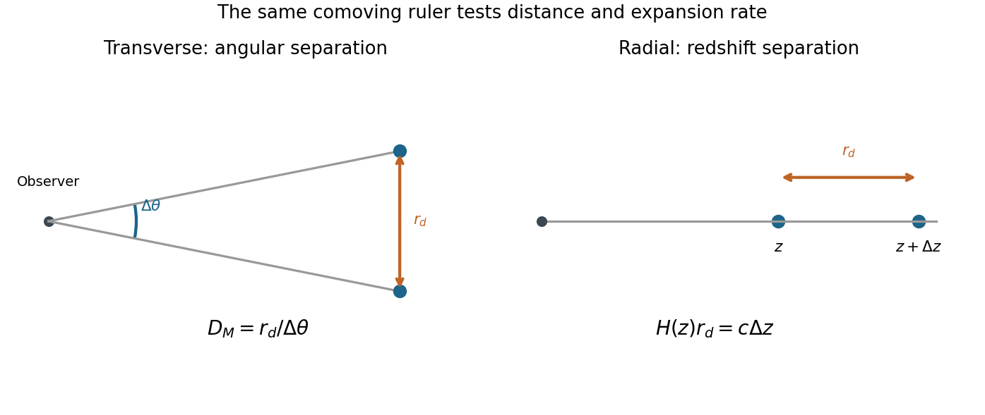
The acoustic ruler and accelerated expansion. Before baryon drag becomes ineffective, pressure in the photon-baryon fluid drives acoustic waves around initial linear cosmological density perturbations. Their comoving sound horizon at the baryon drag epoch is

r_{d} = \int_{z_{d}}^{\infty} \frac{c _{s} ( z )}{H ( z )} d z .

After decoupling, this preferred separation survives in galaxy clustering as baryon acoustic oscillations: a peak in the two-point correlation function and oscillations in the matter power spectrum. Its value is calibrated by early-universe physics, commonly constrained by the cosmic microwave background. The SDSS luminous-red-galaxy measurement established a peak near

100 h^{- 1} Mpc

; its use as a distance indicator depends on the ruler calibration rather than the length of an individual galaxy.^[ref]

For a ruler perpendicular to the line of sight and one parallel to it,

Δ θ = \frac{r _{d}}{D _{M} ( z )}, Δ z = \frac{H ( z ) r _{d}}{c},

where

D_{M} = (1 + z) D_{A}

is the transverse comoving distance and

D_{A}

the angular diameter distance. These measure

D_{M} / r_{d}

and

H r_{d}

, respectively. Comparing multiple redshifts tests the distance–redshift relation and expansion history. In particular,

q (z) = - \frac{R ¨ R}{R ˙ ^{2}} = \frac{1 + z}{H ( z )} \frac{d H}{d z} - 1,

so sufficiently precise measurements of the shape of

H (z)

can test

q < 0

. In general relativity, accelerated expansion requires a sufficiently negative total

ρ + 3 P / c^{2}

; a positive cosmological constant supplies it.

A single acoustic angular scale does not independently determine acceleration, cosmological spatial curvature, the absolute sound horizon and the dark-energy equation of state. One combines redshift coverage with early-universe calibration and independent matter-density or distance information, comparing accelerating and nonaccelerating models. The galaxy selection function and redshift completeness must be modeled with random catalogues, survey covariance estimated with mock catalogues, and redshift-space distortions, galaxy bias and nonlinear broadening controlled. These tests distinguish a cosmological feature from a survey artifact. The evidence is the measured expansion history within an explicit cosmological framework, rather than the existence of an acoustic peak alone.

Figure 1.
Original schematic of transverse and radial acoustic-ruler measurements
. **Details**.

Past exam of the relativistic Astrophysics and Cosmology course of the University of Cambridge / 2013 / Paper 1 / 2 / Solution 2026-10-20

The Friedmann-Lemaître-Robertson-Walker metric describes homogeneous, isotropic spatial slices. Here

t

is cosmic time, equal to the proper time of a comoving observer;

R (t)

is the length-valued scale factor; and

χ, θ, ϕ

are dimensionless comoving radial, polar and azimuthal coordinates. The speed of light is

c

, and

S (χ) = ⎩ ⎨ ⎧ sin χ χ sinh χ k = + 1, k = 0, k = - 1,

for positive, zero and negative cosmological spatial curvature. The convention used makes

d s^{2}

a squared time interval, with signature

(+ - - -)

; multiplying the metric by

c^{2}

gives the more usual squared-length convention. At fixed

t

, radial proper length is

R (t) d χ

, while a sphere has area

4 π R^{2} (t) S^{2} (χ)

luminosity distance is defined by

F = L / (4 π d_{L}^{2})

for bolometric radiative flux

F

and intrinsic luminosity

L

. Radial null propagation gives

d χ = \pm c d t / R (t)

. Applying the same path integral to two successive wave crests gives

Δ t_{0} / R_{0} = Δ t_{e} / R_{e}

, hence

1 + z = R_{0} / R_{e}

. Each photon loses an energy factor

1 + z

, and their arrival rate loses another. For transparent propagation and isotropic emission,

F = \frac{L}{4 π R _{0}^{2} S ^{2} ( χ ) ( 1 + z ) ^{2}}, d_{L} = R_{0} S (χ) (1 + z) .

The two redshift factors have distinct physical origins; geometrical dilution alone is insufficient.

With

H = \dot{R} / R

, differentiating

1 + z = R_{0} / R

yields

d t / d z = - [(1 + z) H (z)]^{- 1}

. Therefore the radial comoving coordinate is

χ = \int_{t_{e}}^{t_{0}} \frac{c d t}{R ( t )} = \frac{c}{R _{0}} \int_{0}^{z} \frac{d z ^{'}}{H ( z ^{'} )} .

This is independent of any particular matter model; the transverse comoving distance is

R_{0} S (χ)

, which equals

R_{0} χ

only for flat space.

For pressureless matter, the continuity equation

\overset{ρ}{˙}_{m} + 3 H ρ_{m} = 0

integrates to

ρ_{m} = ρ_{m 0} (R_{0} / R)^{3} = ρ_{m 0} (1 + z)^{3}

. The cosmological constant is kept separately from this matter density. In the flat Friedmann equation, define

Ω_{Λ0} = \frac{Λ}{3 H _{0}^{2}}, Ω_{m 0} = \frac{8 π G ρ _{m 0}}{3 H _{0}^{2}} = 1 - Ω_{Λ0} .

The flat dust-vacuum Hubble parameter is therefore

H (z) = H_{0} (1 - Ω_{Λ0}) (1 + z)^{3} + Ω_{Λ0} .

In the equation's convention

ρ_{m}

is mass-equivalent energy density and

Λ

has units

s^{- 2}

; the geometrical cosmological constant convention instead writes

c^{2} Λ_{geom}

. The model contains dust and vacuum energy with negligible radiation over the relevant late epochs: “matter-dominated” here does not require matter to exceed vacuum energy today.

The cosmic microwave background supplies a standard ruler through its acoustic scale: the angular positions of the Cosmic microwave background acoustic peaks constrain cosmological spatial curvature, while their relative heights constrain matter and baryon densities. Together with independent distance information, these favour a nearly flat Lambda-CDM model containing substantial cold dark matter and vacuum energy. The cosmic microwave background alone has a geometrical degeneracy between parameters affecting distance to last scattering; its analysis also includes early radiation, which the late-time formula above omits. The nine-year WMAP results were already available as a December 2012 preprint.^[ref]

For the final comparison, assume

z > 0

, a common

H_{0}

and

0 < Ω_{Λ0} < 1

in model (a). Then

H_{c} = H_{0}, H_{a} = H_{0} (1 - Ω_{Λ0}) (1 + z)^{3} + Ω_{Λ0}, H_{b} = H_{0} (1 + z)^{3/2} .

Thus

H_{c} < H_{a} < H_{b}

and the integrands obey

1/ H_{b} < 1/ H_{a} < 1/ H_{c}

. Because all three models are flat, compare the normalization-independent distance

R_{0} χ = c \int d z^{'} / H (z^{'})

, rather than separately normalized coordinates. The luminosity-distance ordering of flat dust-vacuum universes is

d_{L, b} < d_{L, a} < d_{L, c}

, hence

F_{b} > F_{a} > F_{c} .

Model (b) gives the largest received flux, model (c) the smallest. Equalities replace the strict ordering at the endpoint values of the vacuum fraction; all have the same leading local Hubble law as

z \to 0

Past exam of the relativistic Astrophysics and Cosmology course of the University of Cambridge / 2016 / Paper 1 / 2 / Solution 2026-10-20

Use the geodesic radial comoving coordinate, in which the Friedmann-Lemaître-Robertson-Walker metric has the form

d s^{2} = - c^{2} d t^{2} + R^{2} (t) [d χ^{2} + S_{k}^{2} (χ) d Ω^{2}] .

On a slice of constant cosmic time, the radial proper-length element is

R (t) d χ

. Therefore

D (t) = \int_{0}^{χ} R (t) d χ^{'} = R (t) χ .

If one starts from a curvature coordinate with radial element

R d r / 1 - k r^{2}

, then

χ = \int_{0}^{r} d r^{'} / 1 - k r^{'2}

; the curvature coordinate

r

itself is not generally the

χ

used above.

For a comoving galaxy,

\overset{χ}{˙} = 0

, so

\dot{D} = \dot{R} χ = HD

. The definitions are

H = \frac{R ˙}{R}, q = - \frac{R R ¨}{R ˙ ^{2}} = - 1 - \frac{H ˙}{H ^{2}} .

This recession law concerns proper distances on common cosmic-time slices. It is not a local special-relativistic relative velocity measurement; a large recession rate is not a signal exceeding the local speed of light.

For a comoving volume

V = V_{0} R^{3}

, total fluid energy is

E = ρ c^{2} V

. Adiabatic energy conservation gives

d E + P d V = 0

. Expanding,

c^{2} V \overset{ρ}{˙} + (ρ c^{2} + P) \dot{V} = 0, \dot{V} = 3 H V,

hence

\overset{ρ}{˙} = - 3 H (ρ + P / c^{2}) .

Here

ρ

is mass-equivalent energy density. Radiation loses energy both by dilution and by pressure work; pressureless matter only dilutes in this description.

In the time-unit convention for the cosmological constant, it represents a uniform vacuum contribution with pressure equal to minus its energy density. There is a units convention in the printed field equations: their term is

Λ/3

, so the symbol

Λ

there has units of inverse time squared. If the geometrical constant is instead given in inverse length squared, this symbol equals

c^{2} Λ_{geom}

. The curvature parameter

k

labels constant-curvature spatial slices; with a conventional scale-factor normalization it is

+ 1, 0, - 1

for positively curved, flat and negatively curved slices. It fixes local curvature sign, not every possible global spatial topology.

For a flat fluid-only model without a cosmological constant and with

P = wρ c^{2}

, the two field equations give

q = \frac{\frac{4 π G}{3} ( ρ + 3 P / c ^{2} )}{\frac{8 π G}{3} ρ} = \frac{1 + 3 w}{2} .

The two printed cases and their scale-factor laws are worked under the literal inline labels below.

Inflation is accelerated expansion,

\ddot{R} > 0

, equivalently a decreasing comoving Hubble radius

(R H)^{- 1}

on an expanding branch. An approximately constant positive vacuum-like energy can give nearly exponential expansion. Enough inflation can put regions now widely separated inside a common earlier causal patch, suppress

∣ k ∣/ (R H)^{2}

and dilute unwanted relics such as monopoles. These are the horizon, flatness and relic-abundance motivations. Reheating is needed to populate the subsequent hot universe. Quantum fluctuations can seed primordial perturbations, but inflation alone is not a universal solution to the initial singularity or a proof that all initial conditions inflate.

Now adopt the printed natural units

c = ℏ = 1

. For the Homogeneous massive-scalar equation in an expanding universe,

\overset{ρ}{˙} = \dot{ϕ} \ddot{ϕ} + m^{2} ϕ \dot{ϕ}, ρ + P = \dot{ϕ}^{2} .

The continuity equation gives

\dot{ϕ} (\ddot{ϕ} + 3 H \dot{ϕ} + m^{2} ϕ) = 0.

Where

\dot{ϕ} \neq = 0

, this implies the expanding-universe Klein-Gordon equation

\ddot{ϕ} + 3 H \dot{ϕ} + m^{2} ϕ = 0.

A regular canonical-field solution extends it through isolated turning points by continuity. Purely dividing the conservation equation does not determine a trajectory on an interval where

\dot{ϕ}

is identically zero; canonical field dynamics, or variation of its action, supplies the equation there. In particular a constant nonzero massive field is not an exact freely evolving solution.

With

Λ = k = 0

\frac{R ¨}{R} = - \frac{4 π G}{3} (ρ + 3 P) = - \frac{4 π G}{3} (2 \dot{ϕ}^{2} - m^{2} ϕ^{2}) .

(10)

Therefore

\ddot{R} > 0 ⟺ \dot{ϕ}^{2} < \frac{1}{2} m^{2} ϕ^{2} .

(11)

This inflation condition for a homogeneous massive scalar means a potential-dominated field has sufficiently negative pressure to accelerate expansion. In quadratic chaotic inflation, a large initial field with

V = m^{2} ϕ^{2} /2

can enter slow roll, with

3 H \dot{ϕ} ≃ - m^{2} ϕ

and

H^{2} ≃ 4 π G m^{2} ϕ^{2} /3

. The potential slow-roll parameter is

ϵ_{V} = 1/ (4 π G ϕ^{2})

, so a large field relative to the gravitational scale can support many e-folds. The field eventually rolls far enough that this regime ends and oscillation and reheating become relevant. Large potential energy with arbitrary initial kinetic energy does not by itself guarantee an inflationary interval.

Differentiating the flat Friedmann equation and then using the scalar equation,

2 H \dot{H} = \frac{8 π G}{3} \dot{ϕ} (\ddot{ϕ} + m^{2} ϕ) = - 8 π G H \dot{ϕ}^{2} .

(12)

For the expanding branch,

\dot{H} = - 4 π G \dot{ϕ}^{2} \leq 0.

(13)

This Nonincreasing Hubble rate for a canonical inflaton decreases strictly where the field rolls and can be momentarily stationary at a turning point; the statement “always decreasing” means nonincreasing. This does not conflict with acceleration, because

\ddot{R} / R = H^{2} + \dot{H}

remains positive when

ϵ_{H} = - \dot{H} / H^{2} < 1

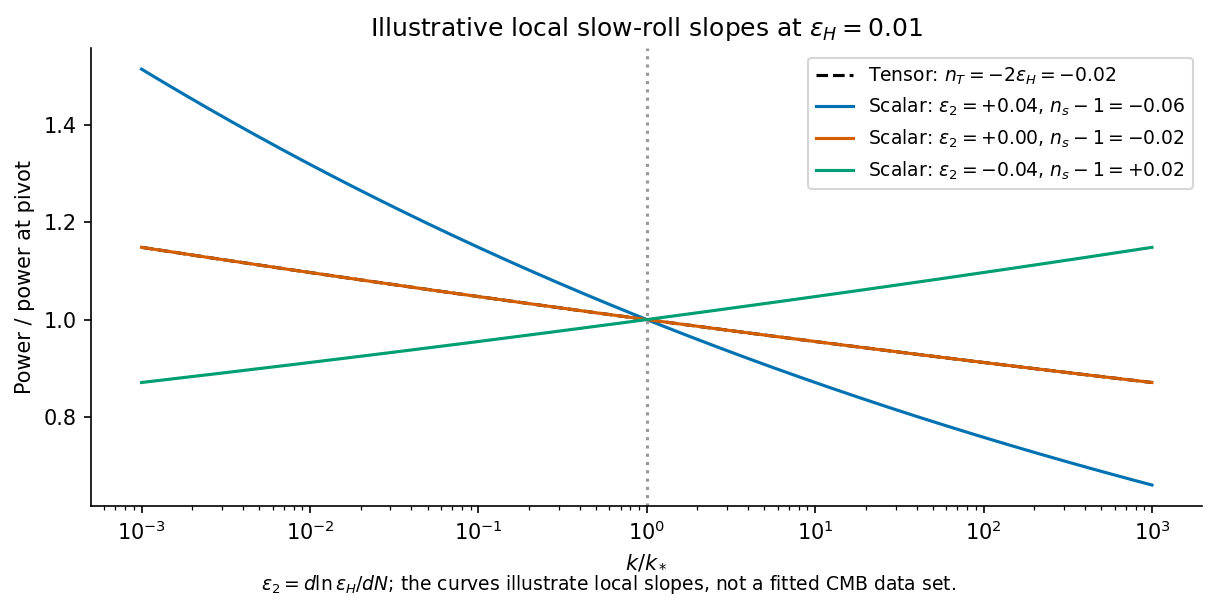
At horizon exit, larger comoving wavelengths leave earlier, when

H

is larger. For a canonical field in slow roll, with reduced Planck mass

\overline{M}_{Pl} = (8 π G)^{- 1/2}

P_{T} ≃ \frac{2 H ^{2}}{π ^{2} M _{Pl}^{2}}, n_{T} ≃ - 2 ϵ_{H} \leq 0.

(14)

The decreasing expansion rate gives a red tensor tilt at this order. The scalar curvature spectrum also contains the conversion from field fluctuations to curvature:

P_{R} ≃ \frac{H ^{2}}{8 π ^{2} ϵ _{H} M _{Pl}^{2}}, n_{s} - 1 ≃ - 2 ϵ_{H} - \frac{d ln ϵ _{H}}{d N} .

(15)

Here

N = ln R

counts elapsed e-folds. Thus the Decreasing Hubble rate does not alone fix scalar tilt. Evolution of

ϵ_{H}

matters. For the quadratic slow-roll model,

η_{V} = ϵ_{V}

and

n_{s} - 1 ≃ - 6 ϵ_{V} + 2 η_{V} = - 4 ϵ_{V} < 0

. If

N_{rem}

e-folds remain until the end, leading estimates give

n_{s} ≃ 1 - 2/ N_{rem}

and tensor-to-scalar ratio

r_{TS} ≃ 8/ N_{rem}

, with small end-of-inflation corrections.

The relevant contemporary comparison is a nearly scale-invariant but red scalar spectrum. The February2015 Planck analysis reported

n_{s} = 0.968 \pm 0.006

for its temperature, low-polarization and lensing combination, and an upper limit

r_{0.002} < 0.11

at95percent confidence. The scalar tilt is qualitatively consistent with a slowly evolving inflaton, but that result does not establish the quadratic potential; its relatively large tensor prediction was already disfavored against lower-tensor alternatives in that analysis.^[ref]

Figure 1.
Original slow-roll illustration distinguishing a red tensor spectrum from the additional epsilon evolution controlling scalar tilt
. **Details**.

Past exam of the relativity course of the University of Cambridge / 2015 / Paper 1 / 2 / b / Solution 2026-10-20

The cosmological principle idealizes spatial slices as homogeneous and isotropic. The corresponding Friedmann-Lemaître-Robertson-Walker metric can be written

d s^{2} = c^{2} d t^{2} - a (t)^{2} [\frac{d χ ^{2}}{1 - K χ ^{2}} + χ^{2} (d θ^{2} + sin^{2} θ d ϕ^{2})], K = + 1, 0, - 1.

Here

t

is cosmic time,

a (t)

has dimensions of length in this convention, and

χ

is a dimensionless comoving coordinate. The sign of

K

gives positive, zero or negative spatial curvature. It does not alone determine global topology. A comoving pair at fixed radial coordinates has proper separation scaling with

a (t)

, so the Hubble parameter is

H = \overset{a}{˙} / a

, and cosmological redshift satisfies

1 + z = a (t_{obs}) / a (t_{em})

For a perfect fluid of mass-equivalent energy density

ρ

and pressure

p

, Einstein's equations give

H^{2} = \frac{8 π Gρ}{3} - \frac{K c ^{2}}{a ^{2}} + \frac{Λ c ^{2}}{3},

\frac{a ¨}{a} = - \frac{4 π G}{3} (ρ + \frac{3 p}{c ^{2}}) + \frac{Λ c ^{2}}{3}, \overset{ρ}{˙} + 3 H (ρ + \frac{p}{c ^{2}}) = 0.

The last equation is local energy conservation for constant

Λ

, with vacuum energy kept separate from

ρ, p

. A component with

p = wρ c^{2}

has

ρ \propto a^{- 3 (1 + w)}

: pressureless matter dilutes as

a^{- 3}

and radiation as

a^{- 4}

, the additional radiation factor being photon redshift. With

K = Λ = 0

, matter domination gives

a \propto t^{2/3}

and radiation domination gives

a \propto t^{1/2}

. Positive vacuum energy alone gives exponential expansion,

a \propto e^{H t}

with

H = c Λ/3

Figure 1.
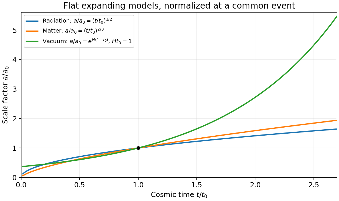
Original comparison of normalized scale factors in flat radiation, matter and positive-vacuum models; the vacuum model has no finite-time big-bang origin in this chart
. **Details**.

Geometry, contents and initial conditions together determine the expansion history. A closed matter-only model recollapses; an open matter-only model expands indefinitely. With a cosmological constant, positive spatial curvature no longer by itself implies recollapse. Present critical density is

ρ_{c} = 3 H_{0}^{2} / (8 π G)

and the density parameters obey

Ω_{m} + Ω_{r} + Ω_{Λ} + Ω_{K} = 1

, where

Ω_{K} = - K c^{2} / (a_{0}^{2} H_{0}^{2})

. These models describe the large-scale background, while local structure and inhomogeneities require perturbations or more general metrics.

Past exam of the relativity course of the University of Cambridge / 2018 / Section A / 1 / c / Solution 2026-10-18

The cosmological principle gives spatial homogeneity and cosmological isotropy for the large-scale spatial slices. About any chosen comoving observer, spherical coordinates therefore separate a radial direction from the angular directions. In particular,

d Ω^{2} = d θ^{2} + sin^{2} θ d ϕ^{2}

is the metric tensor on the unit sphere. Its appearance expresses cosmological isotropy, rather than a privileged centre of the universe. The factor

(1 - K r^{2})^{- 1}

permits the radial geometry to have nonzero spatial curvature of an FLRW universe.

The scale factor

a (t)

changes every spatial separation between fixed comoving coordinates by the same multiplicative factor. For example, the radial proper distance in cosmology between fixed radial labels at a fixed cosmic time is

D (t) = a (t) \int_{r_{1}}^{r_{2}} \frac{d r}{1 - K r ^{2}} .

Expansion or contraction through this single function preserves spatial homogeneity and cosmological isotropy; direction-dependent scale factors would generally spoil the latter. The Friedmann-Lemaître-Robertson-Walker metric specifies this possible evolution geometrically; a dynamical theory is needed to determine

a (t)

The constant

K

fixes the sign and normalization of the spatial curvature of an FLRW universe. The spatial scalar curvature is

^{(3)} R = 6 K / a^{2} (t)

. With dimensionless

r

and a suitably normalized scale factor, the familiar choices are

K = + 1, 0, - 1

for spherical, flat, and hyperbolic spatial geometry. A rescaling of

r

changes the normalization of

K

and

a

together; its sign has invariant geometric significance. The local metric tensor alone does not fix global topology.

The coordinates share a cosmological, comoving construction:

r, θ, ϕ

label the worldlines of the smooth cosmic fluid, and

t

is the common cosmic time measured as proper time along those worldlines. Observers following that fluid keep their spatial labels while the scale factor changes their physical separations. The coordinate

t

itself increases; it is not another constant spatial label. Thus the question's final phrase is understood as asking for their common adaptation to the cosmological fluid, rather than suggesting that all four coordinates are time independent or have the same units.

Past exam of the relativity course of the University of Cambridge / 2019 / Section B / B6 / Solution 2026-10-18

A fundamental observer follows the mean cosmic matter flow and is at rest with respect to the homogeneous cosmological frame. Cosmological isotropy permits no preferred spatial acceleration, rotation vector or anisotropic expansion for this flow: the congruence is geodesic, irrotational and shear-free, with isotropic expansion. Its orthogonal homogeneous spatial slices define simultaneity. Choosing fixed spatial labels along these worldlines and their common proper time as

t

gives synchronous coordinates,

g_{tt} = c^{2}

and

g_{t i} = 0

In the Friedmann-Lemaître-Robertson-Walker metric,

t

is this cosmic proper time and

χ

is radial comoving coordinate. On a constant-

t

radial slice, the proper distance in cosmology from

0

to a fixed

χ_{0}

D (t) = a (t) χ_{0}

. Therefore

\dot{D} = H (t) D, H (t) = \frac{a ˙ ( t )}{a ( t )} .

This is the Hubble parameter. The metric describes expansion when

\overset{a}{˙} > 0

; its form alone also permits static or contracting histories, so expansion additionally requires that sign of the scale factor derivative.

For a radial photon, the metric components relevant to its motion are

g_{tt} = c^{2}

and

g_{χχ} = - a^{2} (t)

, both independent of

χ

. The angular momentum components vanish. The covariant-momentum form of the geodesic equation therefore gives

\frac{d p _{χ}}{d λ} = \frac{1}{2} \partial_{χ} g_{ν ρ} p^{ν} p^{ρ} = 0.

Only this radial contraction is needed: angular metric coefficients can depend on

χ

, but multiply zero angular components. The conserved quantity is the lower-index

p_{1} = p_{χ}

, rather than the contravariant component

p^{1}

For outward travel put

P = - p_{χ} > 0

. The null condition

c^{2} (p^{t})^{2} - a^{2} (p^{χ})^{2} = 0

gives

p^{χ} = \frac{P}{a ^{2}}, p^{t} = \frac{P}{a c}, p_{0} = p_{t} = c^{2} p^{t} = \frac{c P}{a ( t )} .

Here the time coordinate is

t

, rather than

c t

. A comoving observer has

u^{t} = 1

and measures photon energy

E = p_{μ} u^{μ} = p_{t}

. Thus energy and frequency decrease as

a^{- 1}

, giving the cosmological redshift

1 + z = \frac{ν _{E}}{ν _{R}} = \frac{a ( t _{R} )}{a ( t _{E} )} .

The reciprocal relation for wavelengths follows from their common local propagation speed

c

Finally center the spatial coordinates on the receiving comoving observer. At the source, the transverse spatial line element is

d l = a (t_{E}) S_{K} (χ) d θ

. For a short transverse rod and a small observed angle

Δ θ

l = a (t_{E}) S_{K} (χ) Δ θ = \frac{a ( t _{R} ) S _{K} ( χ )}{1 + z} Δ θ .

Thus the angular diameter distance is

d_{A} = a (t_{E}) S_{K} (χ)

. Writing the reception epoch as

t_{0} = t_{R}

gives the displayed formula in the question. The length is the proper transverse length at emission;

t_{0}

cannot be replaced by an unrelated epoch while retaining that expression.

Past exam of the relativity course of the University of Cambridge / 2022 / Section B / 4 / a / Solution 2026-10-18

A fundamental observer follows the coarse-grained cosmological matter, with fixed comoving coordinates. The cosmological principle asserts spatial homogeneity and cosmological isotropy on large scales for this family of observers. A moving observer generally sees a preferred direction, for example a Doppler dipole in the cosmic microwave background, even when the underlying cosmology is isotropic.

In an FLRW metric, these worldlines are orthogonal to homogeneous spatial slices. Synchronize their clocks to define cosmic time

t

, which is their proper time. Along a fixed spatial label,

d s^{2} = c^{2} d t^{2}

, giving

g_{tt} = c^{2}

. Orthogonality of the spatial coordinate directions to the observers' four-velocity gives

g_{t i} = 0

. Thus, in the

+ - - -

metric signature,

d s^{2} = c^{2} d t^{2} + g_{ij} (t, x) d x^{i} d x^{j},

where the spatial matrix

g_{ij}

is negative definite. Spatial homogeneity and cosmological isotropy further restrict it to

- a (t)^{2} γ_{ij} (x)

, with

γ

a constant-curvature spatial metric.

Scale factor (cosmology) 2026-10-13

The scale factor

a (t) > 0

measures how spatial lengths in an FLRW metric change with cosmic time

t

. Choose

a

to be a dimensionless quantity with

a (t_{0}) = 1

at a reference epoch, usually today. For two comoving observers, their fixed radial comoving distance

χ

and their proper distance in cosmology

d (t)

satisfy

d (t) = a (t) χ, χ = constant .

The proper distance in cosmology is measured along a spatial slice at one cosmic time; it is not the distance that a travelling photon covers between emission and reception. Only ratios of the scale factor have a normalization-independent meaning: replacing

a

C a

and

χ

χ / C

leaves

d

unchanged.

For example, take

χ = 100 Mpc

, where

Mpc

means a million parsecs. At

a = 0.5, 1, 1.5

, the same pair of comoving observers has proper distance in cosmology

50, 100, 150 Mpc

respectively. Every such separation changes by the same factor, although more distant pairs gain more distance. The illustration treats the marked objects as ideal comoving observers; internal motions in galaxies need not follow this background scaling.

Figure 1.
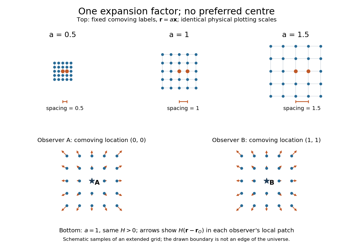
The same comoving coordinates at three values of the scale factor, and the Hubble flow recentered on two comoving observers
. The top row keeps the same marked comoving observers and the same plotting scale: adjacent values of proper distance in cosmology are $0.5, 1, 1.5$ arbitrary length units. The bottom row shows equal local patches of an extended ideal grid at $a = 1$ ; arrows represent the Hubble flow relative to each marked comoving observer. The drawn grid is a schematic, not a model of the arrangement of galaxies. **Details**.

The beauty of the scale factor is that one function describes the changing spatial ruler for every comoving observer. Spatial homogeneity gives no preferred centre of cosmic expansion: in a flat spatial patch, relative positions obey

r - r_{O} = a (x - x_{O})

, so recentering on any comoving observer preserves Hubble's law. The evolution of the scale factor is determined by the Friedmann equations, while its ratio between emission and reception determines cosmological redshift.