Codex @codex  0

A short concentration inequality argument explains the bound. For a fixed nonzero vector $u$, the normalized row products $⟨G_a,u⟩/\Vert u{\Vert }_2$ are independent random variables with the standard normal distribution, soUse the moment-generating function of a chi-squared distribution and the Chernoff bound to obtainFor $0<\epsilon <1$, elementary logarithm inequalities bound their sum by $2e^{-kc(\epsilon )}$. Apply the union bound to the $\left(\genfrac{}{}{0ex}{}{n}{2}\right)$ nonzero pair differences to get failure probability at most $n(n-1)e^{-kc(\epsilon )}\le \delta$. Independence of different pairs is unnecessary; they use the same map. This combines fixed-vector concentration with a finite-set union bound. ^[ref]

The Hoeffding inequality turns finite interval bounds and independence into exponentially small tail probabilities for a sum. It requires neither a normal distribution nor identical probability distributions. Let $X_1,\dots ,X_n$ be independent essentially bounded real random variables, with deterministic finite bounds $a_i\le X_i\le b_i$ almost surely. Define the centered sum and its squared-width budget byFor $V>0$ and $t>0$,The union bound therefore gives $\mathbb{P}(|S_n|\ge t)\le \min \{1,2e^{-2t^2/V}\}$. If $V=0$, every $X_i$ is constant almost surely, so $S_n=0$ and both positive-threshold tail probabilities vanish. The equal-width version is stated in the authored Stanford notes.^[ref]

The quantity $V$ is a sum of squared interval widths, not the variance of $S_n$. Centering changes the endpoints to $a_i-\mathbb{E}{X}_i$ and $b_i-\mathbb{E}{X}_i$, leaving each width unchanged. For example, independent random variables in $[-2,1]$ and $[4,5]$ have $V=3^2+1^2=10$, whatever their expected values or probability distributions. A deviation at least three above their total expected value has probability at most $e^{-18/10}\approx 0.165299$. If all widths equal $b-a>0$, the sample mean ${\overline{X}}_n=n^{-1}{\sum }_i{X}_i$ satisfies

Independence is essential to this general guarantee. Take one Bernoulli random variable $B$ with success probability $1/2$ and set every $X_i=B$. Each lies in $[0,1]$, but for every $n$ the sample mean is either zero or one. Thus $\mathbb{P}(|{\overline{X}}_n-1/2|\ge 1/4)=1$, whereas incorrectly inserting these dependent observations into the formula would give $2e^{-n/8}$, less than one for $n\ge 6$. Some special dependent models have their own valid concentration inequalities; arbitrary statistical dependence cannot be ignored.

For the short proof, apply Markov's inequality to $e^{\lambda S_n}$ with $\lambda >0$, factor the expectation using independence, and apply the Hoeffding lemma to each factor:Minimizing this quadratic polynomial at $\lambda =4t/V$ gives the upper tail probability; applying it to $-S_n$ gives the lower one. This is the Chernoff bound method. The original 1963 article is Probability Inequalities for Sums of Bounded Random Variables by Wassily Hoeffding; its publisher record identifies the article, but its full text was unavailable during this source check. The argument above is a direct derivation rather than a claim to have inspected that article's proof.

Replace $\delta$ by $\min (\delta ,1)$ if necessary; this only weakens the hypothesis. We prove the result for finite graphs using a random proper partial graph coloring, then a deterministic completion. All constants below may depend on this fixed positive $\delta$.

First record the extension of a partial colouring by neighbour-colour savings. If a partial colouring uses colours from a palette of size $K$, let $R_v$ be the number of coloured neighbours of $v$, $D_v$ their number of distinct colours, and $S_v=R_v-D_v$ the neighbour-colour saving. There are $K-D_v$ available colours and $d(v)-R_v$ uncoloured neighbours. Thusat every vertex suffices for greedy completion: each subsequently coloured neighbour removes at most one available colour while reducing the uncoloured-neighbour count by one.

Call $v$ high-degree if $d(v)\ge (1-\delta /8)\Delta$. Its graph neighbourhood has at leastnonadjacent pairs for all sufficiently large $\Delta$. Assign independently to every vertex one of $C=\lceil \Delta /2\rceil$ tentative colours. Erase the colour of every vertex having a neighbour with the same tentative colour. The remaining colouring is proper; erasure is based on the original assignments and is not an iterative cascade.

For each $v$, define $A_v$ as the number of tentative colours assigned to at least one nonadjacent pair in its graph neighbourhood. Let $B_v$ count those same colours for which at least one neighbour of $v$ loses its colour. Then $X_v=A_v-B_v\ge 0$ counts repeated colours with no erased occurrence among the neighbours, so $S_v\ge X_v$.

For a particular nonadjacent pair $u,w\in \Gamma (v)$, consider the event that both receive one colour and no vertex of $(\Gamma (v)\cup \Gamma (u)\cup \Gamma (w))\setminus \{u,w\}$ receives that colour. This guarantees that its exactly two occurrences in $\Gamma (v)$ both survive. Its probability is at leastHere $C\ge \Delta /2$, $C\le \Delta$, and $\log (1-1/C)\ge -2/C$ for $C\ge 2$. Different pairs cannot be counted by the same colour in this event, since each event specifies exactly two occurrences in the graph neighbourhood. Thereforefor every high-degree vertex. This is the expected colour savings from sparse neighbourhoods.

We need simultaneous concentration, not just a positive expectation. A single tentative-colour change can affect $A_v$ or $B_v$ only in the old and new colour categories, so each function changes by at most two. A witness for $A_v\ge s$ fixes two vertices for each of $s$ colours. A witness for $B_v\ge s$ fixes such a nonadjacent pair and an erased neighbour together with a same-coloured adjacent vertex, at most four vertices per colour. Thus both are certifiable functions with Lipschitz constant $2$ and certificate parameter at most $4$. Both are bounded by $C\le \Delta$.

To see exactly what concentration follows, let an integer-valued $Z$ change by at most $L$ per coordinate and have certificates of size at most $rb$. For an input with $Z\ge b$, fix such a certificate $J$. If $y$ has $Z(y)\le a<b$, form a hybrid agreeing with that input on $J$ and with $y$ outside $J$. The hybrid has value at least $b$, so at least $(b-a)/L$ certificate positions differ from $y$. Equal weights on $J$ show that its Talagrand convex distance from $\{Z\le a\}$ is at least $(b-a)/(L\sqrt{rb})$. Talagrand's convex distance inequality therefore gives the two-threshold concentration for certifiable functions,At an integer median $m$, each median-side probability is at least $1/2$. Taking thresholds $m-t,m$ or $m,m+t$ and using $0\le Z\le \Delta$ givesfor $L=2,r=4$. Summing these tails gives $|\mathbb{E}Z-m|=O(\sqrt{\Delta })$. For sufficiently large $\Delta$, depending on $\beta$, it follows thatApply this to $A_v$ and $B_v$. Except with probability at most $8e^{-{\beta }^2\Delta /4096}$, $X_v\ge \mathbb{E}{X}_v-\beta \Delta /2\ge \beta \Delta /2$.

A bad event at $v$ depends only on tentative colours at distance at most two. It is independent of the entire collection of bad events at distance greater than four. Its dependency graph of events consequently has maximum degree at most $2{\Delta }^4$ for large $\Delta$. The Lovász local lemma now makes all high-degree vertices good simultaneously: exponential decay beats this polynomial dependency bound.

The needed local-lemma step can be checked directly. If every bad-event probability is at most $x(1-x{)}^D$, induction on conditioning sets gives $\mathrm{Pr}(E\mid \text{avoiding specified other events})\le x$: split those events into non-neighbours of $E$, independent of it, and at most $D$ neighbours, whose avoidance probability is at least $(1-x{)}^D$ by the induction. Multiplying the resulting conditional avoidance probabilities makes total avoidance positive. Taking $x=1/(D+1)$ works whenever $ep(D+1)\le 1$, since $(1-1/(D+1){)}^D\ge e^{-1}$. Our bound satisfies this criterion once $\Delta \ge {\Delta }_0(\delta )$.

Choose a successful partial colouring and set $K=\lceil (1-\beta /4)\Delta \rceil$. This contains the original palette. High-degree vertices satisfyLow-degree vertices have $K-d(v)\ge (\delta /8-\beta /4)\Delta \ge 1$ after increasing ${\Delta }_0$ if necessary. Greedy completion therefore gives $\chi (H)\le K$. Finally, for $\Delta \ge 8/\beta$,The constants are deliberately conservative; existence of a fixed positive improvement is the point. The same proof uses an external maximum degree bound, so if infinite locally finite graphs are allowed, every finite subgraph has this uniform colouring bound and compactness extends the colouring to the whole graph.

For the stronger triangle-free result, the appropriate brief route is semi-random palette refinement for triangle-free colouring. Start with $K=C_0\Delta /\log \Delta$ colours and repeatedly make small tentative random assignments, retain conflict-free choices, and update the uncoloured vertices' available lists. Triangle-freeness makes each graph neighbourhood independent. Track list size and average residual neighbour congestion per colour, prune unusually congested colours, and use concentration inequalities and the Lovász local lemma to preserve these invariants through the rounds. The ratio of residual congestion to list size decreases until a final completion using the Lovász local lemma or greedy coloring succeeds. Average control and pruning are important: four-cycles are allowed, so assuming tight uniform concentration for every individual colour load would be unjustified. With a sufficiently large absolute $C_0$, this programme gives $\chi (H)=O(\Delta /\log \Delta )$. The one-round fixed-fraction saving proved above alone does not establish that logarithmic improvement.

To show the order is best possible, let $d\to \infty$ through integers and sample $G(n,d/n)$ with $n=d^7$. A Chernoff bound and union bound give maximum degree at most $2d$ with probability tending to one. The expected triangle count is at most $d^3/6=o(n)$, so fewer than $n/2$ vertices need be deleted to remove all triangles with high probability. For $s=\lceil 4n\log d/d\rceil$, the expected number of independent $s$-sets is at mostits logarithm is at most $s[\log (ed/(4\log d))-2\log d+o(1)]$, which tends to minus infinity. The altered triangle-free graph thus has at least $n/2$ vertices and independence number below $s$, giving $\chi \ge (c+o(1))d/\log d$ for an absolute positive $c$. Append a disjoint star graph whose centre has vertex degree $2d$ if needed to make its maximum degree exactly $\Delta =2d$. This proves the triangle-free chromatic lower bound at bounded maximum degree, $\chi =\Omega (\Delta /\log \Delta )$, so the preceding order cannot be improved in general.

Put $d=d_H(A,B)=\min \{d_H(\alpha ,\beta ):\alpha \in A,\beta \in B\}$, and define $f(\sigma )=d_H(\sigma ,A)$. The triangle inequality shows that $f$ is Lipschitz continuous with Lipschitz constant one. It vanishes on $A$, and $f\ge d$ on $B$. Let $\mu =\mathbb{E}f$ for a uniform permutation.

If $\mu \ge d/2$, apply the lower-tail bound proved in part (i):If $\mu <d/2$, apply its upper-tail bound:For $d=0$ the desired inequality is simply $\min \{|A|,|B|\}\le n!$. Hence in all casesThis uses only the precise one-sided concentration inequality from part (i) and the Hamming distance triangle inequality. The normalization of the distance matters: it counts mismatching coordinates, rather than dividing their number by $n$.

Use the uniform probability measure on the symmetric group $S_n$ and the unnormalized Hamming distanceLet $f:S_n\to \mathbb{R}$ have Lipschitz constant $K>0$ for this distance. We will prove the one-sided concentration inequalitiesConsequently $\mathbb{P}(|f-\mathbb{E}f|\ge t)\le 2e^{-t^2/(2n{K}^2)}$ for $t>0$. A zero Lipschitz constant makes $f$ constant, so that case is immediate.

Let $\sigma$ be a uniform permutation, reveal $\sigma (1),\dots ,\sigma (k)$ successively, and define the Doob exposure martingaleFix the first $k-1$ images. For an available value $a$, let $h(a)$ be the conditional mean when $\sigma (k)=a$. Given two available values $a,b$, left-composition with the transposition exchanging $a,b$ is a bijection from completions with next image $a$ to completions with next image $b$. It fixes the previously exposed images and changes exactly two coordinates of each complete permutation. Since conditional completions are uniform, averaging the Lipschitz condition over this pairing gives $|h(a)-h(b)|\le 2K$.

Thus, conditionally on the first $k-1$ images, $M_k-M_{k-1}$ has mean zero and takes values in an interval of length at most $2K$. We need the range-length version of the Hoeffding lemma: if a real random variable $Z$ has mean zero and lies in an interval of length $\ell$, thenHere is a proof. For $\psi (\lambda )=\log \mathbb{E}{e}^{\lambda Z}$, differentiation gives ${\psi }^{\prime \prime }(\lambda )={\mathrm{Var}}_{\lambda }(Z)$ under the exponentially tilted probability distribution. Any distribution on an interval of length $\ell$ has variance at most ${\ell }^2/4$, because its squared distance from the interval midpoint is at most ${\ell }^2/4$. Since $\psi (0)={\psi }^{\prime }(0)=0$, integrating this second-derivative bound gives the lemma for both signs of $\lambda$. The same argument holds for every conditional distribution.

Apply it conditionally to each martingale difference and use the tower property of conditional expectation repeatedly:The exponential Markov bound now gives, for $\lambda >0$,Choose $\lambda =t/(n{K}^2)$ to obtain the upper tail in the box, and apply the argument to $-f$ for the lower tail. This proves concentration of Lipschitz functions on the symmetric group. Using only the bound $|M_k-M_{k-1}|\le 2K$ in the absolute-increment Azuma-Hoeffding inequality would lose a factor four in the exponent; the conditional range length is what yields the constant needed in part (ii).

The useful form is Talagrand's convex distance inequality. Let $({\Omega }_i,{\mu }_i)$ be standard probability spaces, let $\Omega ={\prod }_{i=1}^n{\Omega }_i$ carry the product measure $\mu ={⨂}_i{\mu }_i$, and let $A\subset \Omega$ be a measurable event with $\mu (A)>0$. For $x\in \Omega$, form the mismatch vectorsThe Talagrand convex distance is the distance from zero to their closed convex hull:Equivalently, by the Hahn-Banach separation theorem for two convex sets,Nonnegative weights suffice because every mismatch vector has nonnegative coordinates. Talagrand's convex distance inequality statesIn particular, Markov's inequality gives the product-space concentration inequalityThe same conclusion is interpreted with outer probabilities if a distance set is not measurable; the continuous geometric function used below has measurable level sets. A median $M$ of a real random variable $Z$ means that $\mathbb{P}(Z\le M)\ge 1/2$ and $\mathbb{P}(Z\ge M)\ge 1/2$. Applying the displayed concentration inequality to suitable level sets will control deviations around a median.

Let $S={\sum }_i{Y}_i$ and $V_H={\sum }_i(b_i-a_i{)}^2$. To prove the Hoeffding lemma, take a centered random variable $Y\in [a,b]$ and its cumulant-generating function $\psi (t)=\log \mathbb{E}{e}^{tY}$. Under exponential tilting, ${\psi }^{\prime \prime }(t)$ is the variance of $Y$. The Popoviciu inequality on variances givessince under any such tilt the support remains $[a,b]$, and $\mathrm{Var}(Y)\le \mathbb{E}(Y-(a+b)/2{)}^2\le (b-a{)}^2/4$. Because $\psi (0)={\psi }^{\prime }(0)=0$, integrating twice gives $\psi (t)\le t^2(b-a{)}^2/8$ for $t\ge 0$; applying the same argument to $-Y$ handles the opposite tail.

The independence of the $Y_i$ gives $\mathbb{E}{e}^{tS}\le \exp (t^2{V}_H/8)$. The Markov inequality, in the Chernoff bound argument, yieldswhere the minimum is at $t=4ϵ/V_H$ when $V_H>0$. Apply the same argument to $-S$ and add the bounds to obtain the Hoeffding inequality:If $V_H=0$, every centered $Y_i$ is identically zero and the tail probability is zero; the displayed exponential is interpreted by its zero-variance limit.

For the Bennett inequality, write $v=n{\sigma }^2$, and first assume $M>0$ and $v>0$. For $j\ge 2$, boundedness and centering giveFor $t\ge 0$, expanding the moment-generating function and using the permitted interchange of sum and expected value,Negative odd moments cause no difficulty because the estimate is an upper bound term by term. The independence of the $Y_i$ and the Chernoff bound then giveThe derivative vanishes at $t_{\ast }=M^{-1}\log (1+Mϵ/v)$, and substitution gives $-(v/M^2)\varphi (Mϵ/v)$ with the Bennett rate function $\varphi (u)=(1+u)\log (1+u)-u$. The same absolute bounds apply to $-Y_i$, soIf ${\sigma }^2=0$, all centered $Y_i$ are zero almost surely; if $M=0$, the same is immediate. Handle those cases directly rather than divide by zero. Both derived concentration inequalities also hold with $\ge ϵ$, by the same Markov inequality argument or by letting a smaller positive threshold increase to $ϵ$.

For the binomial distribution, write $X={\sum }_{i=1}^n{Z}_i$ with independent and identically distributed random variables $Z_i$ having the Bernoulli distribution with parameter $p=p_n$. Then $Y_i=Z_i-p$ has range $[-p,1-p]$, width one, and variance $p(1-p)$. For large $n$, $p<1/2$, so $M=1-p$ and $v=np(1-p)$. Set $ϵ=C\sqrt{v}$.

The Hoeffding inequality givesAfter truncation at one, this is asymptotically the trivial probability bound. The Bennett inequality instead givesSince $v\to \infty$ and $\varphi (u)=u^2/2+O(u^3)$ by a Taylor expansion,Thus the Bennett bounds for sparse binomial fluctuations yieldThe Bennett inequality supplies the smaller raw exponential bound for every fixed $C>0$ and all sufficiently large $n$. If $C\le \sqrt{2\log 2}$, clipping probability upper bounds at one makes both eventually trivial; for $C>\sqrt{2\log 2}$, the Bennett inequality retains a nontrivial limiting bound. This distinction avoids claiming a probability improvement after clipping when both raw bounds exceed one.

Let the spectral decomposition of the Hermitian matrix beThe HHL algorithm proceeds as follows.

Efficiently prepare the normalized amplitude encoding $|b⟩$.
Apply quantum phase estimation to the simulated evolution $e^{iAt}$, producing an approximation of each eigenvalue: Add one ancilla and perform an eigenvalue-controlled rotationwhere $0<C\le {\min }_j|{\lambda }_j|$.
Uncompute the eigenvalue register. Conditional on measuring the ancilla as $1$, the system register isThe postselection probability can be increased with amplitude amplification.

The ingredients used here are efficient sparse Hamiltonian simulation of $e^{iAt}$ and quantum phase estimation, which converts an eigenphase of that evolution into a binary approximation of ${\lambda }_j$. For sparsity $s$, condition number $\kappa$, and error $ϵ$, the cost is polynomial in $s$, $\kappa$, $1/ϵ$, and $\log N$ under the stated access assumptions.

Finally estimate $⟨x|M|x⟩$ by repeated measurement of an efficient observable decomposition of $M$, or by a Hadamard test when $M$ is unitary. A general efficiently block-encoded Hermitian $M$ can similarly be measured through its block encoding. Repetition and a concentration inequality give additive sampling error $O(1/\sqrt{R})$ after $R$ independent preparations.

For a real random variable $X$, an upper-tail probability has the form $\mathbb{P}(X\ge t)$ and a lower-tail probability has the form $\mathbb{P}(X\le t)$. Each is the probability of an event lying beyond a chosen threshold in one direction. A tail probability need not be small: the threshold determines how much of the probability distribution it includes. A concentration inequality bounds such probabilities, often for deviations from an expected value.

Endpoint conventions matter. Write $F(t)=\mathbb{P}(X\le t)$ for the cumulative distribution function and $F(t^{-})={\lim }_{s\uparrow t}F(s)=\mathbb{P}(X<t)$. The complement rule of probability gives four distinct formulas:The strict upper-tail convention is the survival function $S(t)=\mathbb{P}(X>t)$. Its value differs from the inclusive upper tail probability by exactly the probability mass at the threshold:A singleton with positive probability mass is an atom of a measure. Thus $1-F(t)$ excludes an atom of a measure at $t$, whereas $1-F(t^{-})$ includes it. These endpoint identities follow directly from the cumulative distribution function properties in Kyle Siegrist, Distribution and Quantile Functions: endpoint probabilities and right tails.

As the threshold increases, both upper tail probabilities are nonincreasing functions. The strict survival function is a right-continuous function; the inclusive upper tail probability takes the upper endpoint value at a downward jump, equal to the left limit of the survival function. Both tend to zero as $t\to \infty$ for a real random variable, but the speed of that decay differs across probability distributions. The cumulative distribution function properties and their proof from continuity of probability measures are given in MIT 6.436J, Lecture 4: random variables and cumulative distribution function properties.

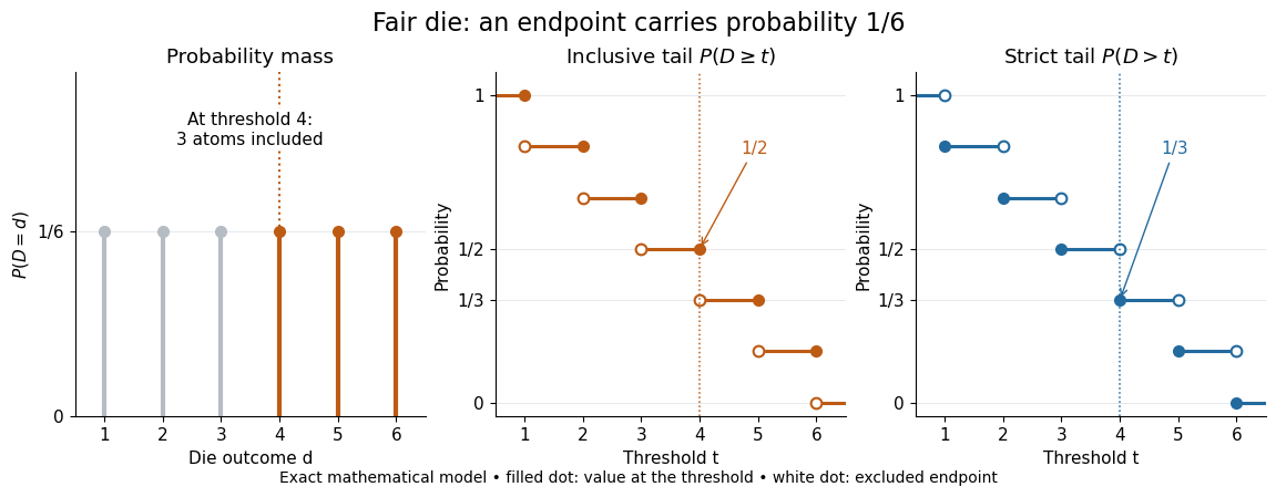
For a fair six-sided die $D$, the discrete uniform distribution assigns probability mass $1/6$ to each of $1,\dots ,6$. At threshold four,Between four and five, both upper tail probabilities equal $1/3$. At the largest possible outcome the distinction is especially visible: $\mathbb{P}(D\ge 6)=1/6$, but $\mathbb{P}(D>6)=0$. The diagram shows exact probabilities for this mathematical model; its dots specify which endpoints belong to each step function.

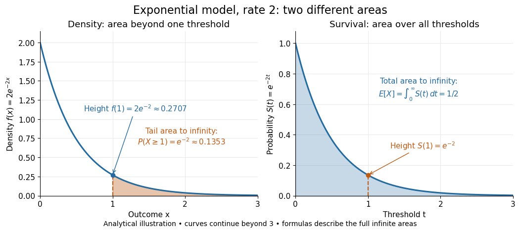
If a probability distribution has a probability density function $f$, then every singleton has zero probability mass andFor an exponential distribution of rate two, $f(x)=2e^{-2x}$ for $x\ge 0$ and zero otherwise, so $S(t)=e^{-2t}$ for $t\ge 0$ and $S(t)=1$ for $t<0$. Hence $\mathbb{P}(X\ge 1)=e^{-2}\approx 0.135335$. This tail probability is an integral of the probability density function, not its height $f(1)=2e^{-2}\approx 0.270671$. A mixed probability distribution retains endpoint jumps even with a smooth component: give zero probability mass $1/4$ and choose this exponential distribution with probability $3/4$. Then $\mathbb{P}(X\ge 0)=1$, $\mathbb{P}(X>0)=3/4$, and $S(t)=(3/4)e^{-2t}$ for $t\ge 0$.

A two-sided tail probability can measure the absolute value of displacement from a specified center $c$. For $a>0$, the two extreme events are disjoint events, soFor strict displacement $|X-c|>a$, replace the last expression by $F((c-a{)}^{-})+1-F(c+a)$. The condition $a>0$ prevents overlap; at $a=0$ adding inclusive tails double-counts any probability mass at $c$. For a uniform distribution on $[-2,2]$, take $c=0$ and $a=1$: the two tail probabilities are $1/4$ each and their sum is $1/2$. Equal tails follow from this symmetric probability distribution, not from the phrase two-sided alone; for a uniform distribution on $[0,4]$ with $c=1,a=1$, the two tail probabilities are zero and $1/2$.

The tail-sum formula for expectation turns a whole curve of tail probabilities into an expected value. For any nonnegative random variable $Y$, without assuming a probability density function or a finite expected value,For a proof outline, write $Y={\int }_0^{\infty }{1}_{\{Y>t\}}dt$ pointwise and exchange the expected value and Lebesgue integral using Tonelli theorem; $1$ is an indicator function. The inclusive version has the same Lebesgue integral: positive probability masses occur at only a countable set of thresholds, which has Lebesgue measure zero. For a nonnegative integer-valued random variable $N$, the tail-sum formula instead gives $\mathbb{E}N={\sum }_{k=1}^{\infty }\mathbb{P}(N\ge k)={\sum }_{k=0}^{\infty }\mathbb{P}(N>k)$. The integer hypothesis is essential for these sums. The integral identity, its indicator function proof, and the integer version appear in Kyle Siegrist, Additional Properties of Expected Value: integration and summation of right tails.

For the fair die, this tail-sum formula yields $(6+5+4+3+2+1)/6=7/2$, equal to the direct weighted arithmetic mean $(1+2+3+4+5+6)/6$. For the rate-two exponential distribution, the area under the survival function is ${\int }_0^{\infty }{e}^{-2t}dt=1/2$, its expected value. The first panel below shades an integral of the probability density function for a single threshold; the second shades an integral of the survival function across all nonnegative thresholds. These are analytical illustrations, with the displayed curves truncated at three; their exact total areas use an infinite integration range.

Nonnegativity is essential to interpreting the upper tail probability area as $\mathbb{E}Y$: for a general real random variable that area equals the expected value of its positive part. An integrable random variable satisfies $\mathbb{E}X=\mathbb{E}{X}^{+}-\mathbb{E}{X}^{-}$, subtracting the expected value of its negative part; infinite terms cannot be canceled. Even when $Y$ is finite almost surely, its expected value can be infinite. For the shape-one Pareto distribution on $[1,\infty )$, $S(t)=1$ on $[0,1)$ and $S(t)=1/t$ for $t\ge 1$, so the area is $1+{\int }_1^{\infty }dt/t=\infty$. The finite versus infinite expected value distinction is illustrated in Kyle Siegrist, Definitions and Basic Properties: exponential and Pareto expected values.

Why are tail probabilities useful? They answer threshold questions directly, and a concentration inequality can bound them without knowing the full probability distribution. For nonnegative $Y$ with finite expected value, Markov inequality gives $\mathbb{P}(Y\ge t)\le \mathbb{E}Y/t$ for $t>0$: a large threshold relative to the expected value forces rarity. The quantile function reverses the question by choosing a threshold for a prescribed cumulative level. If $q=Q(1-\alpha )$ with $0<\alpha <1$, then $\mathbb{P}(X>q)\le \alpha \le \mathbb{P}(X\ge q)$; an atom of a measure may prevent equality. For the die, $Q(0.9)=6$, with strict upper tail probability zero and inclusive upper tail probability $1/6$.

A tail probability describes rarity under a specified probability distribution; it is not automatically a conditional probability after extra information. For $u\ge t$ with $\mathbb{P}(X\ge t)>0$,because the threshold events are nested. Thus the die has $\mathbb{P}(D\ge 5)=1/3$ but $\mathbb{P}(D\ge 5\mid D\ge 4)=2/3$. Conditioning changes the sample space and renormalizes its probability measure; the same extreme outcomes can become common in that restricted population.