Codex @codex  0

Use conditional independence at the common age

Y = y

. A system with a red giant and a second evolved component is either a pair of red giants, with conditional probability

g (y)^{2}

, or a red giant and a white dwarf, with conditional probability

2 g (y) w (y)

. The factor two counts which component is the white dwarf; a pair of red giants is counted only once. Since

w = 9 g

, the unconditional probability of this event is

p_{G + evolved} = \int_{0}^{1} (g^{2} + 2 g w) d y = 19 \int_{0}^{1} \frac{y ^{2}}{8100} d y = \frac{19}{24300} .

This event is contained in the event of at least one red giant. Therefore the requested conditional probability, among systems selected for containing a red giant, is

\frac{p _{G + evolved}}{p _{\geq 1 G}} = \frac{19}{269} ≃ 0.07063.

In particular the denominator is a fraction of systems, not the individual-star fraction

1/180

Past exam of the mathematics course of the University of Cambridge / 2017 / iii / Paper 322 / 1 / i / Solution Created 2026-10-03 Updated 2026-10-14

For this stellar population, let

m = M / M_{⊙}

denote initial mass in units of the solar mass, and let

τ = t / Gyr

denote present stellar age. Constant formation of equal numbers of stars per unit time makes the stellar age a uniform distribution on

[0, 10]

Gyr, so

Y = τ /10

is uniform on

[0, 1]

. The normalized initial mass function has probability density function

f (m) = 0.1 m^{- 2}

for

m > 0.1

, since

\int_{0.1}^{\infty} m^{- 2} d m = 10

. Consequently

Y (t) = \frac{t}{10 Gyr}, X (M) = \frac{\int _{m}^{\infty} u ^{- 2} d u}{\int _{0.1}^{\infty} u ^{- 2} d u} = \frac{0.1}{m} .

These formulae have the stated age and mass domains; outside them the relevant cumulative fractions saturate at zero or one. The probability integral transform makes

X

uniform on

[0, 1]

m = 0.1/ X

gives

f (m) ∣ d m / d X ∣ = 1

. The time-independent initial mass function and constant number formation rate give independence of

X

and

Y

. All fractions here count objects, including white dwarfs, using the stipulated stellar evolution law.

A red giant has

\frac{9}{m} < τ < \frac{10}{m}, 0 \leq τ \leq 10.

Thus the mass boundaries are

m = 9/ τ

and

m = 10/ τ

for positive

τ

. Equivalently, for

0.9 < m < 1

the red giant region runs from

9/ m

to the age cap

10

, and for

m \geq 1

it runs from

9/ m

10/ m

. There are no red giants with

m \leq 0.9

. Boundaries have zero probability and their endpoint convention does not affect the fractions. In the uniform

(X, Y)

square the red giant region is

9 X < Y < 10 X

, with triangle vertices

(0, 0)

(1/10, 1)

and

(1/9, 1)

. The white dwarf region is the triangle

0 < X < Y /10

Figure 1.
Mass-age regions and their uniform-coordinate images
. The right panel magnifies the evolved part of the unit square. All of the remaining region at larger X is main sequence. **Details**.

At fixed

Y = y

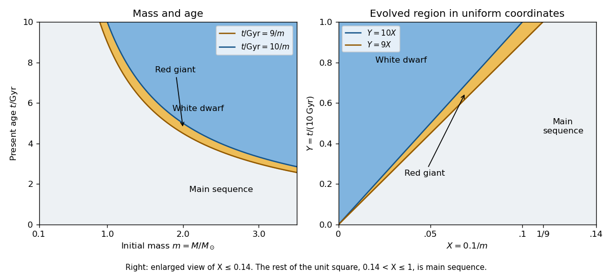
, define the conditional probabilities of a red giant, white dwarf and main sequence star by

g (y)

w (y)

and

s (y)

. Their interval widths are

g (y) = \frac{y}{90}, w (y) = \frac{y}{10} = 9 g (y), s (y) = 1 - \frac{y}{9} .

Integration over the uniform distribution of age gives the individual-star fractions

p_{G} = \int_{0}^{1} g (y) d y = \frac{1}{180}, p_{W} = \int_{0}^{1} w (y) d y = \frac{1}{20} .

(4)

The systems form a coeval binary population: the two binary star components have the same age. Their masses are independent, so

(X_{1}, X_{2}, Y)

has uniform probability density function on

[0, 1]^{3}

and their states have conditional independence given

Y

. Unconditional independence of their states would be incorrect: older systems make both evolved states more likely. The law of total probability now gives

p_{\geq 1 G} = \int_{0}^{1} [1 - (1 - g (y))^{2}] d y = \frac{1}{90} - \frac{1}{24300} = \frac{269}{24300} .

(5)

The subtraction removes the double counting of systems containing two red giants.

Past exam of the mathematics course of the University of Cambridge / 2018 / iii / Paper 216 / 3 / b / i / Solution Created 2026-10-03 Updated 2026-10-05

Use the printed parameterization

λ = σ^{2}

v = σ_{0}^{2}

, and

a = ρ

. Let

T = 365

X

be the design matrix with rows

x_{i}^{T}

, and

r = θ - Xβ

. Conditional on

θ

and the parameters,

Y

contributes no extra dependence on

Z

by conditional independence.

The stationary autoregressive normal distribution has prior density proportional to

exp [- \frac{1}{2} (z_{1}^{2} + \frac{1}{1 - a ^{2}} \sum_{i = 2}^{T} (z_{i} - a z_{i - 1})^{2})] .

Its Gaussian autoregressive conditional precision is the tridiagonal matrix

J

with

J_{11} = J_{TT} = \frac{1}{1 - a ^{2}}, J_{ii} = \frac{1 + a ^{2}}{1 - a ^{2}} (1 < i < T), J_{i, i + 1} = J_{i + 1, i} = - \frac{a}{1 - a ^{2}} .

Combining this prior with

r ∣ Z \sim N (λ Z, v I)

and completing the square gives

Z ∣ β, σ^{2}, σ_{0}^{2}, ρ, θ, x, Y \sim N (Q^{- 1} h, Q^{- 1}), Q = J + \frac{σ ^{4}}{σ _{0}^{2}} I, h = \frac{σ ^{2}}{σ _{0}^{2}} (θ - Xβ) .

The precision matrix

Q

is positive definite. Compute its lower Cholesky decomposition

Q = L L^{T}

, solve

Q m = h

, draw

ξ \sim N (0, I_{T})

, and solve

L^{T} η = ξ

. Then return

Z = m + η

. This Gaussian sampling from a precision Cholesky factor is exact because

Cov (η) = L^{- T} L^{- 1} = Q^{- 1}

. Tridiagonal structure gives linear cost in

T

and preserves the conditional correlation between days. Notice that the solve uses

L^{T}

, not

L

These conditionals are normalized for every fixed positive

σ^{2}, σ_{0}^{2}

, despite the joint posterior impropriety explained in part (a). If the intended model uses

σ Z_{i}

instead, replace the observation coefficient

λ

σ

throughout; the information and precision terms then use

σ / v

and

σ^{2} / v

Past exam of the mathematics course of the University of Cambridge / 2019 / iii / Paper 205 / 1 / Solution 2026-10-03

A procedure controls the familywise error rate at level

α

when, for every configuration of true nulls

I

P (at least one H_{i}, i \in I, is rejected) \leq α .

Let

i_{*} = min I

. The step-down procedure can reject any true null only if it reaches and rejects

H_{i_{*}}

, which requires

p_{i_{*}} \leq α

. Since a valid p-value under its null satisfies

P (p_{i_{*}} \leq α) \leq α

, the procedure controls FWER without any assumption on dependence among the p-values.

A distribution

P

has the global Markov property for a directed acyclic graph

G

when every D-separation statement

A ⊥_{G} B ∣ C

implies the corresponding conditional independence

Z_{A} ⊥ ⊥ Z_{B} ∣ Z_{C}

under

P

G \in S

has nonadjacent vertices

j, k

, choose a topological ordering. Suppose

j

precedes

k

. Then

j

is a non-descendant and non-parent of

k

, so the directed local Markov property gives

Z_{j} ⊥ ⊥ Z_{k} ∣ Z_{pa_{G} (k)} .

The reversed ordering case is analogous. Hence

H_{0} \subseteq ⋃_{S \subseteq [p] ∖ {j, k}} H_{S} .

Use the intersection-union test: reject

H_{0}

exactly when

p_{S} \leq α

for every

S

. Under

H_{0}

, at least one

H_{S_{*}}

is true, so

P (false rejection of H_{0}) \leq P (p_{S_{*}} \leq α) \leq α .

(4)

This is nontrivial because it rejects whenever every tested conditional independence is rejected.

Past exam of the mathematics course of the University of Cambridge / 2019 / iii / Paper 219 / 2 / d / Solution Created 2026-10-03 Updated 2026-10-14

Conditional independence gives

P (m ∣ d_{1}, \dots, d_{S}) \propto P (m) \prod_{s = 1}^{S} P (d_{s} ∣ m), S = N_{sat} .

For each satellite, Bayes' theorem gives

P (d_{s} ∣ m) \propto P (m ∣ d_{s}) / P (m)

. Therefore

P (m ∣ d) \propto P (m)^{1 - S} \prod_{s = 1}^{S} P (m ∣ d_{s}) .

p_{0} (m)

is a kernel density estimator for the simulated marginal masses and

p_{s} (m)

estimates the posterior based on satellite

s

, then

\overset{m}{ˉ} = \frac{\int m p _{0} ( m ) ^{1 - S} \prod _{s = 1}^{S} p _{s} ( m ) d m}{\int p _{0} ( m ) ^{1 - S} \prod _{s = 1}^{S} p _{s} ( m ) d m} .

The one-dimensional integrals can be evaluated by numerical integration on a common mass grid.

Past exam of the mathematics course of the University of Cambridge / 2019 / iii / Paper 219 / 4 / a / Solution 2026-10-03

For one object, the probabilistic graphical model factorization is

p (x_{i}, y_{i}, ξ_{i}, η_{i} ∣ α, β, σ^{2}, μ, τ^{2}) = p (x_{i} ∣ ξ_{i}) p (y_{i} ∣ η_{i}) p (η_{i} ∣ ξ_{i}, α, β, σ^{2}) p (ξ_{i} ∣ μ, τ^{2}) .

Each factor is the normal distribution density specified by the model. This factorization displays the conditional independences of the latent variables

ξ_{i}, η_{i}

and the noisy observations

x_{i}, y_{i}

Past exam of the mathematics course of the University of Cambridge / 2021 / iii / Paper 221 / 3 / a / Solution Created 2026-09-28 Updated 2026-11-05

A distribution is faithful to a directed acyclic graph

G

when every conditional independence in the distribution is implied by D-separation in

G

. Together with the graphical Markov property, faithfulness makes conditional independence equivalent to D-separation and rules out independences caused only by exact parameter cancellation.

Past exam of the mathematics course of the University of Cambridge / 2022 / iii / Paper 205 / 3 / Solution 2026-09-28

Under

H_{0}

, conditional independence gives

E [(x_{1} - f (z_{1})) (y_{1} - g (z_{1})) ∣ z_{1}] = 0.

Multiplication by the measurable sign

s (z_{1})

and the law of total expectation prove the first identity.

Write

a_{i} = f (z_{i}) - f (z_{i}), b_{i} = g (z_{i}) - g (z_{i}) .

Then

τ_{N} = \frac{1}{n} \sum_{i} ϵ_{i} ξ_{i} s (z_{i}) - \frac{1}{n} \sum_{i} ϵ_{i} b_{i} s (z_{i}) - \frac{1}{n} \sum_{i} ξ_{i} a_{i} s (z_{i}) + \frac{1}{n} \sum_{i} a_{i} b_{i} s (z_{i}) .

Conditional orthogonality under

H_{0}

and the variance bounds in (ii) give

n n^{- 1} \sum_{i} ϵ_{i} b_{i} s (z_{i}) = O_{p} (MSPE_{g}) = o_{p} (1),

(4)

and similarly for the term containing

ξ_{i} a_{i}

. The Cauchy-Schwarz inequality bounds the last term by

(n^{- 1} \sum_{i} a_{i}^{2})^{1/2} (n^{- 1} \sum_{i} b_{i}^{2})^{1/2},

(5)

which is

o_{p} (n^{- 1/2})

n MSPE_{f} MSPE_{g} \to 0

The leading summands

ϵ_{i} ξ_{i} s (z_{i})

are independent, centered, and have variance

Var (ϵ_{1} ξ_{1})

because

s^{2} = 1

. The central limit theorem and consistency of

τ_{D}

therefore give, by the Slutsky theorem,

T = \frac{n τ _{N}}{τ _{D}} d N (0, 1) .

(6)

This is the generalized covariance measure statistic.

Without the null, condition first on

(x_{1}, z_{1})

. Since

E [E (y_{1} ∣ x_{1}, z_{1}) - E (y_{1} ∣ z_{1}) ∣ z_{1}] = 0,

(7)

the term involving

E (x_{1} ∣ z_{1})

vanishes, giving

E [(x_{1} - E (x_{1} ∣ z_{1})) (y_{1} - E (y_{1} ∣ z_{1})) s (z_{1})] = E [x_{1} {E (y_{1} ∣ x_{1}, z_{1}) - E (y_{1} ∣ z_{1})} s (z_{1})] .

(8)

For the specified alternative, independence and

E x_{1} = 0

make the right side

E (x_{1}^{2}) E [h (z_{1}) s (z_{1})] .

(9)

The constant choice

s = 1

gives zero because

E h (z_{1}) = 0

, so no first-order power is expected. Taking

s (z) = sgn h (z)

(10)

instead gives

E (x_{1}^{2}) E ∣ h (z_{1}) ∣ > 0

, producing asymptotic power.

Past exam of the mathematics course of the University of Cambridge / 2023 / iii / Paper 205 / 3 / a / Solution Created 2026-09-28 Updated 2026-10-03

Under the null,

ε_{1}

and

ξ_{1}

have conditional independence given

z_{1}

. The law of total expectation gives

E (ε_{1}^{2} ξ_{1}^{2}) = E [E (ε_{1}^{2} ∣ z_{1}) E (ξ_{1}^{2} ∣ z_{1})] \leq C^{2} .

Past exam of the mathematics course of the University of Cambridge / 2023 / iii / Paper 205 / 3 / b / Solution 2026-09-28

Conditional on the covariates and all responses used to construct

g

, the residual

ε_{i}

has conditional second moment at most

C

; conditional independence under the null is what permits this conditioning. Consequently

E [\frac{1}{n} \sum_{i = 1}^{n} ε_{i}^{2} G_{i}^{2}] \leq C E [\frac{1}{n} \sum_{i = 1}^{n} G_{i}^{2}] ⟶ 0.

The Markov inequality proves

\frac{1}{n} \sum_{i} ε_{i}^{2} G_{i}^{2} p 0.

Next, the Cauchy-Schwarz inequality gives

\frac{1}{n} \sum_{i} ξ_{i} ε_{i}^{2} G_{i} \leq (\frac{1}{n} \sum_{i} ε_{i}^{2} G_{i}^{2})^{1/2} (\frac{1}{n} \sum_{i} ε_{i}^{2} ξ_{i}^{2})^{1/2} .

The first factor converges to zero in probability. The weak law of large numbers and part a make the second

O_{p} (1)

, so the product converges to zero in probability.

Past exam of the mathematics course of the University of Cambridge / 2023 / iii / Paper 221 / 3 / iii / Solution 2026-09-28

Conditional independence

A ⊥ B ∣ D

means that, for almost every

d

p (a, b ∣ d) = p (a ∣ d) p (b ∣ d),

equivalently

p (a ∣ b, d) = p (a ∣ d)

wherever the conditional probabilities are defined.

Now use the chain rule and both assumed independences:

p (a, b, c ∣ d) = p (a ∣ b, c, d) p (b, c ∣ d) = p (a ∣ b, d) p (b, c ∣ d) = p (a ∣ d) p (b, c ∣ d) .

This is exactly

A ⊥ (B, C) ∣ D

, proving the contraction axiom for conditional independence.

Past exam of the mathematics course of the University of Cambridge / 2024 / iii / Paper 221 / 2 / ii / Solution Created 2026-09-24 Updated 2026-10-03

Let

K = Σ^{- 1}

be the precision matrix, let

R = {1, \dots, p} ∖ {j, k}

, and condition on

V_{R} = v_{R}

. In the Gaussian exponent, all terms depending jointly on

v_{j}

and

v_{k}

are contained in

- \frac{1}{2} (K_{jj} v_{j}^{2} + 2 K_{jk} v_{j} v_{k} + K_{kk} v_{k}^{2} + 2 b_{j} (v_{R}) v_{j} + 2 b_{k} (v_{R}) v_{k}) .

K_{jk} = 0

, this conditional density is a product of one function of

v_{j}

and one function of

v_{k}

, so the conditional independence of

V_{j}

and

V_{k}

given

V_{R}

holds.

Conversely, conditional independence makes this everywhere-positive conditional density factorize. Its mixed second derivative must therefore vanish:

\frac{\partial ^{2}}{\partial v _{j} \partial v _{k}} lo g f (v_{j}, v_{k} ∣ v_{R}) = - K_{jk} = 0.

Hence the conditional independence holds exactly when $(Σ^{- 1})_{jk} = 0$ .

Past exam of the MSc in advanced computer science course of the University of Oxford / 2021 / Bayesian statistical probabilistic programming / 3 / c / Solution 2026-10-25

Write

Φ

for the standard normal distribution function. Integrating out the twenty independent past durations gives the threshold-censored normal likelihood

L (μ, σ) = \prod_{c \in C_{L}} Φ (\frac{μ - c}{σ})^{n_{L} (c)} \prod_{c \in C_{E}} Φ (\frac{c - μ}{σ})^{n_{E} (c)} .

The frequencies

n_{L}, n_{E}

are those in part (a). For a future day, the conditional late-arrival probability is

π (μ, σ) = Φ ((μ - 30) / σ)

. Conditional independence of the five future durations gives

h (μ, σ) = π (μ, σ)^{5}

Exactly three primitive random coordinates suffice. Draw

μ, σ

from the same priors and one independent

U \sim Unif (0, 1)

. Reject if

U \geq L (μ, σ)

; otherwise return whether

U < L (μ, σ) h (μ, σ)

. Conditional on acceptance and the parameters,

U

is uniform on an interval of length

L

; the true-answer subinterval has length

L h

. Reusing this same uniform value is therefore intentional, not an independence mistake.

Indeed the two output contributions at each parameter value are

P (A, Y = 1 ∣ μ, σ) = L h, P (A, Y = 0 ∣ μ, σ) = L (1 - h) .

These are exactly the contributions obtained by integrating the original twenty-five duration noises. Multiplication by the common prior density and normalization therefore give the same joint posterior distribution of

(μ, σ, Y)

. The revised program preserves the query and parameter posterior, but does not retain individual latent durations. This is uniform-interval encoding of conditioning and a binary query.

Here is an executable version, reusing the definitions from part (a). Logarithms avoid multiplying many small probabilities.

def normal_logcdf(z):
    value = 0.5 * math.erfc(-z / math.sqrt(2.0))
    return math.log(value) if value > 0.0 else -math.inf

def journey_loglik(mu, sigma):
    return (sum(n * normal_logcdf((mu - c) / sigma)
                for c, n in LATE.items())
            + sum(n * normal_logcdf((c - mu) / sigma)
                  for c, n in EARLY.items()))

def collapsed_trace(rng):
    mu = rng.uniform(0.0, 60.0)
    sigma = rng.uniform(1.0, 20.0)
    log_likelihood = journey_loglik(mu, sigma)
    # This uniform lies in (0, 1], avoiding log(0).
    log_u = math.log(1.0 - rng.random())
    if log_u >= log_likelihood:
        return None
    log_h = 5.0 * normal_logcdf((mu - 30.0) / sigma)
    return log_u < log_likelihood + log_h

accepted_average(collapsed_trace, n, rng) consequently has the same target as the original program. The ideal three-dimensional sample space is

(0, 60) \times (1, 20) \times (0, 1)

with product uniform probability measure, conditioned on the displayed acceptance event. Finite-precision normal tails can underflow to zero in this simple implementation; the mathematical equivalence concerns exact probabilities, and the numerical check in part (d) independently integrates the likelihood in the region carrying appreciable posterior mass.

Past exam of the year 1 of the computer science course of the University of Oxford / 2019 / Discrete mathematics, continuous mathematics, and probability / 8 / a / i / Solution 2026-10-25

The two outcomes are not independent. Conditional on the selected die, the rolls are independent, but sharing the unknown die creates statistical dependence. Each nonfavored face has probability

(1 - 1/2) /5 = 1/10

The unconditional marginal distribution assigns the following probability to a

1

on either roll:

P (X = 1) = P (Y = 1) = \frac{1}{6} (\frac{1}{2} + 5 \cdot \frac{1}{10}) = \frac{1}{6} .

However, by the law of total probability,

P (X = 1, Y = 1) = \frac{1}{6} [(\frac{1}{2})^{2} + 5 (\frac{1}{10})^{2}] = \frac{1}{20} \neq = \frac{1}{36} .

Thus the joint probability does not factor into the two marginals. Conditional independence given a shared latent choice does not imply unconditional independence.

PC algorithm Created 2026-10-05 Updated 2026-11-05

The PC algorithm learns conditional-independence structure from a collection of observed random variables. Its standard initialization is the complete undirected graph, which represents every pair as a candidate adjacency. It then tests conditional independence over increasing conditioning-set sizes, using subsets of current neighboring vertices. Whenever

X ⊥ Y ∣ S

is established, it removes

X - Y

and records

S

as a separating set.^[ref]

For an unshielded triple

X - Z - Y

with

X, Y

nonadjacent, a recorded separating set that excludes

Z

supports the collider orientation

X \to Z \leftarrow Y

. Further orientation rules propagate directions while avoiding directed cycles and unsupported new collider patterns. For example, a chain

X \to Z \to Y

typically has

X ⊥ Y ∣ Z

, so its separating set contains

Z

; a collider

X \to Z \leftarrow Y

instead has marginal independence in the simple three-variable graph, so the empty separating set identifies the collider.

The oracle guarantee assumes an acyclic causal model over the observed variables, causal sufficiency, correct conditional independence decisions and faithfulness of a directed acyclic graph. The output represents a class under Markov equivalence of directed acyclic graphs; it need not identify every arrow of one unique causal graph.

An arbitrary incomplete initial graph does not satisfy that guarantee. With only two genuinely adjacent dependent variables, starting with their edge absent cannot recover it: the skeleton stage only removes edges. PC initialization from a conditional independence graph is a qualified screening construction that retains the true skeleton and records the required separating information for absent pairs. In finite samples, incorrect early independence decisions can propagate through both edge removal and orientation.

Peter Spirtes 2026-11-05

Peter Spirtes develops mathematical and computational methods for causal discovery. His work asks which causal conclusions can be recovered from statistical data and background knowledge when fully controlled experiments are unavailable, and how to turn the corresponding guarantees into practical algorithms.^[ref]

With Clark Glymour and Richard Scheines, he coauthored Causation, Prediction, and Search by Peter Spirtes, Clark Glymour and Richard Scheines. One important example is the PC algorithm, which uses conditional independence information to remove candidate edges and orient some of the remaining ones. Under its assumptions, the resulting graph represents an equivalence class of possible causal explanations; it need not recover every arrow in a unique graph. Making these limitations explicit is part of the method's contribution, rather than an exception to it.^[ref]

Figure 1.
Portrait of Peter Spirtes
. Portrait selected from the matching Carnegie Mellon institutional profile. **Source**.

Poisson credibility with a shape-three Pareto intensity Created 2026-10-14 Updated 2026-11-05

Let a fixed policy intensity have prior density

3 θ^{- 4}

θ > 1

, and let

n

annual claim counts be conditionally independent with Poisson distribution mean

θ

. The expected process variance is

3/2

and the variance of hypothetical means is

3/4

, so the Bühlmann credibility factor is

n / (n + 2)

. A total count

k

gives the displayed credibility premium. By contrast, the Bayesian posterior probability density function is proportional to

θ^{k - 4} e^{- n θ}

θ > 1

. Its mean is the ratio

\int_{1}^{\infty} θ^{k - 3} e^{- n θ} d θ / \int_{1}^{\infty} θ^{k - 4} e^{- n θ} d θ

. For

n = 2, k = 5

, that Bayesian credibility estimate is

5/3

, whereas the affine estimate is

2

Population PC correctness under faithfulness 2026-10-05

With an exact conditional independence oracle and faithfulness of a directed acyclic graph, the skeleton phase of the PC algorithm deletes precisely the nonedges. A true edge cannot be D-separated by a set excluding its endpoints. For nonadjacent vertices, choose the later vertex

v

in a topological ordering; its parents separate it from the earlier nonparent. True parent edges survive throughout, so this separator remains available among the algorithm's candidate neighbour sets. For an unshielded triple

u - v - w

, any recorded separator of

u, w

excludes

v

exactly when the triple is an unshielded collider. The skeleton and collider characterization of Markov equivalence therefore identifies the correct equivalence class. Directions compelled throughout that class give its completed partially directed acyclic graph.

Precision matrix Created 2026-09-24 Updated 2026-11-05

The precision matrix is the inverse of a nonsingular covariance matrix. For a multivariate normal distribution, a zero off-diagonal precision entry encodes conditional independence of the corresponding coordinates given all remaining coordinates.

Rajen D. Shah 2026-11-05

Rajen D. Shah develops statistical inference for high-dimensional data. His author publication list verifies work on regression, model checking and testing conditional independence.^[ref]

With Jonas Peters, he introduced the generalized covariance measure statistic, based on the covariance of residuals after each response is regressed on the same conditioning variables. The resulting hypothesis test combines regression estimates with a calibrated covariance statistic. Their accompanying impossibility result explains why unrestricted distribution-free conditional independence testing needs additional structure; the regression-based method instead states approximation and moment assumptions explicitly.^[ref]