Codex @codex  0

Write the magnetic flux linkage of the stationary pickup coil as $\lambda ={\sum }_{n=1}^N{\Phi }_n$, in SI units of weber. If every turn links the same magnetic flux $\Phi$, then $\lambda =N\Phi$; the turn count is dimensionless. With a fixed winding and terminal convention, Faraday's law of induction gives the induced electromotive forceThis is the fundamental theorem of calculus applied to magnetic flux linkage. Its units are $\mathrm{V}\mathrm{s}=\mathrm{Wb}$, not volts alone. Reversing the leads reverses the sign. In a high-input-electrical resistance voltage measurement the input approximately follows this electromotive force; coil loading and the frequency response of the electronics require separate calibration.

Separate direct drive linkage from material linkage: $\lambda ={\lambda }_{\mathrm{drive}}+{\lambda }_{\mathrm{material}}$. Even an empty pickup coil has $-d{\lambda }_{\mathrm{drive}}/dt$. In an ideal long, uniformly coupled specimen with negligible demagnetizing field correction and eddy current shielding, a useful material approximation isHere $A_s$ is specimen cross-sectional area, not the larger coil aperture; ${\mu }_0$ is vacuum permeability and $M$ the axial magnetization sampled by the coil. The units check directly: $(\mathrm{V}s/(\mathrm{A}\mathrm{m}))({\mathrm{m}}^2)(A/m)=\mathrm{V}\mathrm{s}$. Finite geometry and nonuniform magnetization generally require a calibrated coupling in place of ${\mu }_{0}N{A}_s$. The exact linkage identity survives that failure of the uniform approximation.

As an original illustrative calculation, stipulate $N=100$, $A_s=10^{-6}{\mathrm{m}}^2$, $\Delta M=10^{3}A/m$ and rounded ${\mu }_0=4\pi \times 10^{-7}\mathrm{V}s/(\mathrm{A}\mathrm{m})$. ThenA uniform change over $0.10\mathrm{ms}$ would give a rectangular pulse of $-1.25664\mathrm{mV}$; over $0.20\mathrm{ms}$ it gives $-0.628319\mathrm{mV}$ with the same area. Thus pulse height mixes change size with change speed. These numbers describe an ideal model, not observed pulses or material constants.

The two-state calculation is not a general formula for a ferromagnet. Exchange interactions, magnetic domains, magnetic domain-wall pinning, magnetic anisotropy, and hysteresis can determine which response is accessible. Both spin angular momentum and orbital angular momentum can contribute; a single constant gyromagnetic ratio may be only a restricted effective description. Rotation sets an internal bias, while the material and its preparation determine magnetization. The Barkhausen effect illustrates why a smooth bias can produce jumps instead of the toy smooth curve.

For a limited, reversible, isotropic linear model, suppose the same intrinsic volume magnetic susceptibility ${\chi }_v$ responds to the applied bias and to $B_{\Omega }/{\mu }_0$. For a uniformly magnetized ellipsoid along a principal axis, include its demagnetizing factor $N_d$:Solving this linear equation yieldsHere $H_{\mathrm{int}}$ and $H_{\mathrm{app}}$ are actual magnetic field intensities; the added rotational bias is an equivalent drive in the constitutive response. In SI, dimensionless ${\chi }_v$ multiplies an intensity in $A/m$, so $M_z={\chi }_v\Omega /\gamma$ would omit ${\mu }_0$ and have the wrong units. A susceptibility defined instead as $\partial M/\partial B$ has different units. State the convention before comparing formulas.

At zero applied magnetic field intensity, a stipulated ${\chi }_v=3$ gives prefactor $3/2$ in a sphere, with $N_d=1/3$, and a prefactor approaching $3$ in a long axial ellipsoid. This is a geometry check of the assumed linear model. A real cylinder does not have an exactly uniform demagnetizing field, and an irreversible ferromagnet cannot in general be represented by this single linear equation. Inferring an intrinsic gyromagnetic ratio requires an independently calibrated material response and a geometry-dependent conversion of the measured stray magnetic field.

A demagnetizing factor relates a component of demagnetizing field to magnetization. The three principal factors of a uniformly magnetized ellipsoid sum to one in the International System of Units. Factors quoted in a different unit convention need conversion; state the convention and measurement geometry before applying them.

The demagnetizing field is the contribution to magnetic field intensity produced by the sample's own magnetization. Inside a uniformly magnetized ellipsoid, it is uniform and has the form ${\mathbf{H}}_d=-\mathsf{N}\mathbf{M}$; the demagnetizing factor along a principal axis gives its longitudinal component. These conditions make the scalar correction in field conventions for magnetic susceptibility useful.

A cylinder generally has spatially varying magnetization and demagnetizing field. A volume-sensitive instrument and a short central pickup coil consequently need different effective corrections: one averages over the sample, while the other samples central flux. A shape factor copied from an ellipsoid is not an exact correction for every cylinder, especially with nonlinear response or hysteresis. ^[ref]

In vacuum, magnetization is zero and magnetic flux density obeys $\mathbf{B}={\mu }_0\mathbf{H}$. The applied quantities ${\mathbf{H}}_{\mathrm{app}}$ and ${\mathbf{B}}_0={\mu }_0{\mathbf{H}}_{\mathrm{app}}$ mean the field of the external sources at the sample position with the sample absent. The internal magnetic field intensity includes the sample's demagnetizing field; its internal magnetic flux density additionally includes ${\mu }_0\mathbf{M}$. A field quoted in the tesla is a $B$ quantity, even when an instrument informally calls it “$H$”.

For a uniformly magnetized ellipsoid, along a principal axis with demagnetizing factor $N_d$ in the International System of Units,For a sphere, $N_d=1/3$. The axial value approaches zero in the long slender ellipsoid limit and the normal value approaches one in the thin flat ellipsoid limit. Thus a stipulated intrinsic volume magnetic susceptibility ${\chi }_v=3$ would yield apparent values $1.5$ in a sphere and approximately $3$ in a long axial sample. These are calculated geometry effects, not measured material values. For fixed $N_d$, implicit differentiation gives the same conversion for local differential magnetic susceptibility, $dM/d{H}_{\mathrm{app}}={\chi }_{\mathrm{diff}}/(1+N_d{\chi }_{\mathrm{diff}})$.

To isolate finite size from quantum vortex penetration, keep the same weak-field London equations but replace the half-space by an infinite slab $-d/2\le z\le d/2$. Put equal tangential magnetic fields $B_0\hat{\mathbf{x}}$ at its two faces. With $z=0$ now at the slab center, the even solution and its signed current density areThe hyperbolic cosine profile has equal boundary values, while the electric currents on the two sides have opposite signs. In particular,For the stipulated thickness $d=2{\lambda }_L$, the center retains about $0.648B_0$ and the mean is about $0.762B_0$, even though this is a Meissner state. For $d\gg {\lambda }_L$, the center magnetic field is exponentially small and the mean is about $2{\lambda }_L{B}_0/d$, reflecting the two surface layers. For $d\ll {\lambda }_L$, the mean tends to $B_0$: little screening is possible across such a short distance. These are analytic model examples, not material measurements. Real finite objects also need their demagnetizing field and edge geometry accounted for; the slab calculation only isolates the effect of thickness.

A Gouy balance detects the force exerted by a nonuniform magnetic field on a sample of uniform cross-section extending between high- and low-field regions. TeachSpin's implementation reverses the usual arrangement: a rare-earth permanent-magnet assembly sits on a one-pan electronic balance, while a separate holder brings the sample into the field. The magnet's apparent mass change measures the opposite of the sample's vertical force, by Newton's third law. The described pole faces have diameter $25\mathrm{mm}$ and separation $15\mathrm{mm}$; samples occupy cuvettes of cross-section $(10\mathrm{mm}{)}^2$ and height about $32\mathrm{mm}$. ^[ref]

The same balance calibrates magnetic flux density by measuring the reaction force on the magnet when a wire of known horizontal length $L$ carries known electric current $i$ perpendicular to the field: $|F_z|=iL{B}_0$. The manufacturer describes water being repelled by the high-field region, identifying negative magnetic susceptibility. This observed sign supplies a qualitative test, not a measured Curie's law curve. ^[ref]

For weak reversible linear response, a uniform sample displacing a weakly magnetic surrounding medium has, to leading order, downward forceThis follows by integrating the induced-dipole force density $({\chi }_v-{\chi }_{\mathrm{medium}}){\partial }_z(B_0^2)/(2{\mu }_0)$ along a downward coordinate. $A$ is the cross-sectional area, and the two $B_0$ values are applied magnetic flux densities. The force depends on the endpoint fields; the entire field-gradient profile need not be measured under these assumptions. In the reversed apparatus, $F_{\downarrow }=-g\Delta m_{\mathrm{magnet}}$ after subtracting the holder background, where $g$ is gravitational acceleration. This sign must be reversed before inferring volume magnetic susceptibility.

Useful controls are an empty-holder reading at the same position, a distant-sample baseline, repeated wire-current reversals during field calibration, and stable temperature. They separate holder response, balance drift, force offsets, and thermal changes; these are proposed checks for the stated inference. Finite endpoint fields, nonuniform cross-section, uneven powder packing, stray forces and a demagnetizing field limit the simple formula. If magnetization is nonlinear, the weak-response force involves $A{\int }_{B_{0,\mathrm{top}}}^{B_{0,\mathrm{bottom}}}M(B_0)d{B}_0$ instead of a constant-${\chi }_v$ endpoint square. A balance reading then measures an integrated response, not directly the local differential magnetic susceptibility.

For a bulk type-II superconductor with negligible demagnetizing field, raising the applied magnetic field intensity past the lower critical value $H_{c1}$ favors a superconducting mixed state containing quantum vortex lines; superconductivity survives until the upper critical value $H_{c2}$. The magnetic field extends around each vortex over a penetration scale, not solely inside its core. Thus a nonzero average magnetic flux density can coexist with superconductivity. Below $H_{c1}$, a type-II superconductor also supports a Meissner state; a vortex-free state above the equilibrium entry field may instead be metastable. ^[ref]

Real preparation histories may leave quantum vortex lines held in place by material inhomogeneities, retaining magnetic flux and producing hysteresis. This flux pinning restricts access to equilibrium: it is different from the arbitrary frozen interior magnetic field of the ideal perfect conductor model. Harvard's vortex-imaging work illustrates strong pinning to bulk disorder in a type-II superconductor. ^[ref] Separately, flux conservation in a superconducting loop and fluxoid and flux quantization in a superconductor explain why a hole can retain magnetic flux. Neither bore retention, vortex penetration nor weak screening in a thin sample should be silently identified with the equilibrium Planar London screening calculation.

Magnetic susceptibility describes how readily a magnetic field changes a material's magnetization. The field variable and normalization matter: volume magnetic susceptibility in the International System of Units is dimensionless, whereas a derivative of total magnetic moment with respect to $B$ has units of $\mathrm{J}{\mathrm{T}}^{-2}$. A slope measured against the applied magnetic field intensity also depends on the sample's demagnetizing field.

For an isotropic, reversible linear response through the origin, writeHere $\mathbf{M}$ is magnetization, or magnetic moment per volume; ${\mathbf{H}}_{\mathrm{int}}$ is the internal magnetic field intensity; ${\mathbf{B}}_{\mathrm{int}}$ is the internal magnetic flux density; and ${\mu }_0$ is the vacuum permeability. Both $M$ and $H$ have units $\mathrm{A}{\mathrm{m}}^{-1}$. The magnetic permeability is ${\mu }_0(1+{\chi }_v)$. ^[ref]

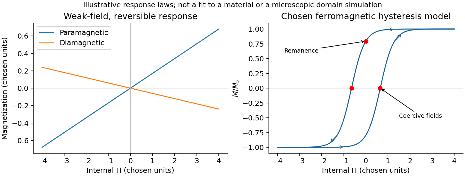
The independent-moment magnetic response below shows why one number cannot describe every field: magnetization approaches a saturation magnetization, while its differential magnetic susceptibility approaches zero. Anisotropy requires a magnetic susceptibility tensor; hysteresis requires specifying the preparation and sweep branch as well as the bias magnetic field, temperature, and timescale. The Gouy balance turns a small response into a measurable force without presuming that its readout is already the intrinsic volume magnetic susceptibility.

Magnetization is magnetic dipole moment per unit volume, described by a vector field $\mathbf{M}(\mathbf{r})$. Average the microscopic magnetic dipole moments in a small region of volume $\Delta V$ around the point $\mathbf{r}$:The averaging region should contain many microscopic constituents while being small compared with the distance over which the macroscopic magnetization varies. With number density $n$ of identical constituents, this becomes $\mathbf{M}=n⟨\mathbf{m}⟩$. Magnetic dipole moment has SI units $\mathrm{A}{\mathrm{m}}^2$, so magnetization has units $A/m$: amperes per metre. The average is a vector sum, not a sum of magnitudes.^[ref]

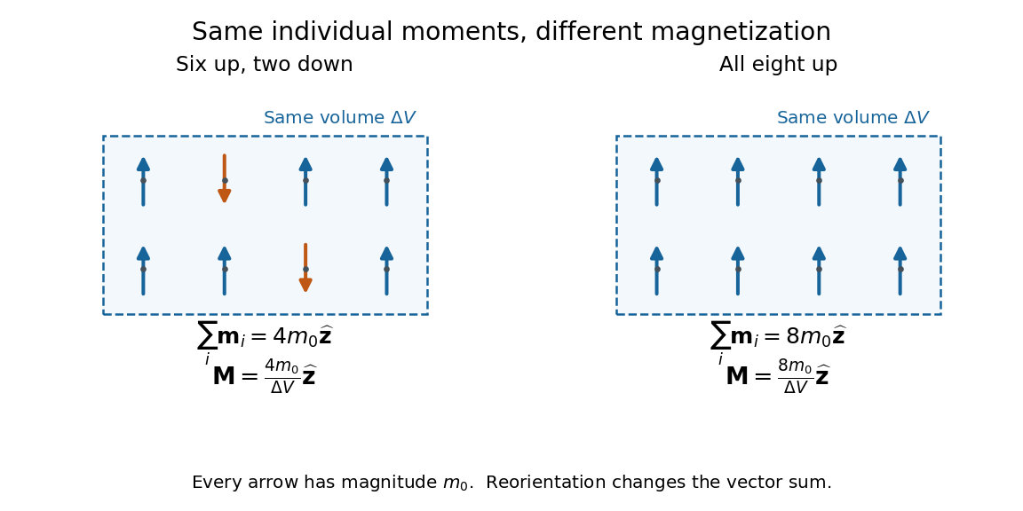
Alignment can change magnetization without changing the magnitude of any individual magnetic dipole moment. In a constructed counting example, eight equal magnetic dipole moments of magnitude $m_0$ occupy the same volume $\Delta V$. Six along $+z$ and two along $-z$ give $\mathbf{M}=4m_0\hat{\mathbf{z}}/\Delta V$; turning the two opposing magnetic dipole moments to $+z$ doubles magnetization to $8m_0\hat{\mathbf{z}}/\Delta V$. Both arrangements have the same sum of magnitudes, $8m_0$. Changing the individual magnetic dipole moments provides another possible response; their alignment and their magnitudes are distinct ingredients. Microscopic spin contributes magnetic dipole moment without being a literal rotating charged ball.

Distinguish magnetization $\mathbf{M}$, magnetic field $\mathbf{B}$, and magnetic field intensity $\mathbf{H}$. In SI,Here ${\mu }_0$ is the vacuum permeability, and $\mathrm{T}$ denotes the tesla. Magnetization describes matter's magnetic dipole moment density; magnetic field enters the Lorentz force; magnetic field intensity separates the free electric current contribution in the macroscopic equations. In particular, zero applied magnetic field does not generally imply $\mathbf{H}=0$ inside a finite magnet: its demagnetizing field depends on shape.^[ref]

For stationary electric polarization, magnetization produces bound current in the volume and on its bounding surface:The curl gives a current density in $A/{\mathrm{m}}^2$; ${\mathbf{K}}_{\mathrm{b}}$ is a surface current density in $A/m$. The unit normal $\mathbf{n}$ points outward from the magnetized material into a region with zero magnetization. Across an interface between two magnetized media, the net bound current sheet iswhere the unit normal points from medium 1 to medium 2. Both faces contribute: medium 2 has the opposite outward normal vector. This fixes the cross product sign. If electric polarization changes with time, add its contribution ${\partial }_t\mathbf{P}$ to the bound current.^[ref]

A short proof outline explains why both contributions are needed. Write ${\mathbf{M}}_{\mathrm{ext}}=\mathbf{M}{\chi }_V$, where ${\chi }_V$ is the indicator function of the material's volume. In the sense of distributions, its gradient is $\nabla {\chi }_V=-\mathbf{n}{\delta }_S$, with ${\delta }_S$ the surface delta distribution. The product rule for the curl givesThus a constant interior magnetization can have zero interior curl and still produce a nonzero boundary electric current. Equivalently, neighboring ideal microscopic current loops cancel along shared edges while uncompensated edges remain on the outside. This bound current representation predicts the same macroscopic magnetic field as the magnetization distribution; it does not require a wire or free charge transport around the magnet. Its usefulness is that the familiar Biot-Savart law can now calculate the magnetic field from a specified magnetization.

A time-dependent average magnetization need not vary smoothly under a smooth drive. The Barkhausen effect resolves collective jumps through their induced electromotive force; Barkhausen pulse area explains how that derivative readout relates to the underlying change.

For a homogeneous linear isotropic sphere in a uniform applied field, the internal field is ${\mathbf{H}}_i={\mathbf{H}}_0-\mathbf{M}/3$. Combining this geometric demagnetizing field with $\mathbf{M}=\chi {\mathbf{H}}_i$ gives the title expression. Matching the scalar magnetic potentials $-H_{i}r\cos \theta$ inside and $-H_{0}r\cos \theta +C\cos \theta /r^2$ outside provides an independent boundary-value derivation. Tangential $H$ is continuous without free surface current and normal $B$ is continuous. A negative susceptibility makes magnetization antiparallel, not parallel in sense, to the applied field.

Write the two allowed moment projections as $\pm \mu$, where $\mu =g{\mu }_B/2$ for spin one-half. Their Zeeman energies in the prescribed flux density are $\mp \mu B$. The single-particle partition function and the mean moment along the field areFor noninteracting moments, magnetization is moment per volume:For electron-like spin-only moments $g\simeq 2$, these become $M_s=N{\mu }_B/V$ and $\eta ={\mu }_B/k_B$.

Differentiate with respect to the specified $B$ to obtainThis $B$ derivative is not a dimensionless SI volume susceptibility. In the weak-feedback approximation $B\simeq {\mu }_{0}H$, the usual dimensionless differential susceptibility is ${\chi }_{\mathrm{diff}}\simeq {\mu }_0{\chi }_B$. The small-field limit gives Curie's law ${\chi }_0={\mu }_{0}N{\mu }^2/(V{k}_{B}T)$. At finite bias a secant response $M/H\simeq {\mu }_{0}M/B={\chi }_0\tanh (x)/x$ differs from the differential slope ${\chi }_0{\mathrm{sech}}^{2}x$. For an internal $B={\mu }_0(H+M)$ retained self-consistently, the exact local conversion is ${\chi }_H={\mu }_0{\chi }_B/(1-{\mu }_0{\chi }_B)$; demagnetizing geometry can further affect an applied-field measurement. Stating the field convention avoids a hidden factor of ${\mu }_0$ or confusion between a slope and a ratio.

For an ideal long specimen with negligible demagnetizing field, the Meissner state has $B={\mu }_0(H+M)=0$, so $M=-H$. A type-I superconductor retains this response up to its thermodynamic critical field $H_c(T)$ and then enters the normal state, where the small normal magnetic response can be neglected. Nonzero demagnetizing fields can create an intermediate state and broaden the measured transition.

A type-II superconductor is fully screening only below $H_{c1}(T)$. Between $H_{c1}$ and $H_{c2}$, magnetic flux enters as quantized vortices and the reversible magnetization remains diamagnetic but decreases in magnitude towards zero at $H_{c2}$. Above $H_{c2}$ the bulk is normal. Ginzburg–Landau theory distinguishes the types at $\kappa =1/\sqrt{2}$, not at $\kappa =1$; the later condition in the source merely restricts its estimate.

The $H$–$T$ sketch has two increasing-width regions below $T_c$: Meissner below the lower boundary, mixed vortex state between the two boundaries, and normal state above the upper boundary. Both critical fields vanish at $T_c$. The phase-diagram panel of the original figure in solution shows this topology; its normalized field curves are illustrative, not a fit to the source magnetization loop.

Along the in-plane hard axis, the ideal uniform-magnetization model gives reversible rotation from the easy direction toward the applied field. With uniaxial anisotropy energy density $K_u{\sin }^2\theta$, minimization givesfollowed by saturation at $\pm M_s$. The right panel of the preceding figure therefore has a nearly linear central section, essentially zero remanence and ideally no hysteresis. Actual domains, misalignment and defects can produce rounding or a small loop. This is an in-plane hard axis; the much larger out-of-plane demagnetizing field is a different effect.

The microscopic magnetic response becomes a macroscopic field problem through the magnetization $\mathbf{M}$, the magnetic dipole moment per unit volume. Definein magnetostatics. Bound currents are represented by ${\mathbf{J}}_b=\nabla \times \mathbf{M}$ and surface current ${\mathbf{K}}_b=\mathbf{M}\times \hat{\mathbf{n}}$. Normal $B$ is continuous across an interface, while $\hat{\mathbf{n}}\times ({\mathbf{H}}_2-{\mathbf{H}}_1)={\mathbf{K}}_{\mathrm{free}}$. It is generally incorrect to impose continuity of every component of both fields. A linear isotropic material has $\mathbf{M}=\chi \mathbf{H}$ and ${\mu }_r=1+\chi$, but a ferromagnet usually requires a nonlinear, history-dependent constitutive relation.

Internal field differs from externally applied field. For uniform magnetization along a principal axis of an ellipsoid, the demagnetizing field is $-N_{d}M$ and $H_{\mathrm{int}}=H_{\mathrm{applied}}-N_{d}M$. A linear specimen therefore has apparent susceptibility $\chi /(1+N_d\chi )$ relative to the applied field. Shape is especially important for large susceptibility. A long closed magnetic circuit reduces stray fields; a bar magnet still has demagnetizing fields despite the absence of magnetic monopoles. Equivalent magnetic-pole descriptions are bookkeeping for magnetization divergence, not free magnetic charge.^[ref]

In paramagnetism, permanent localized moments are preferentially aligned by the field, against thermal disorder. For independent spin-one-half moments with projections $\pm \mu$, the two Zeeman energies givein the dilute weak-field limit with $B\simeq {\mu }_{0}H$. This is a Curie law; the response saturates at $n\mu$ when alignment dominates. More generally, spin $J$ gives $\chi ={\mu }_{0}n(g{\mu }_B{)}^{2}J(J+1)/(3k_{B}T)$. Interactions can produce a Curie–Weiss response $C/(T-\Theta )$ over a suitable range. Conduction-electron Pauli paramagnetism need not show the localized-moment $1/T$ law.

In diamagnetism, the field induces a magnetic moment opposing it, so the linear susceptibility is negative. The microscopic cause is the change in orbital electronic motion, and a closed-shell insulating material has no permanent atomic moment to orient. This weak response is often only mildly temperature dependent away from other transitions. It also exists as a background in materials with a stronger positive response. Perfect flux expulsion in a superconductor is a distinct collective phenomenon and should not be identified with ordinary weak atomic diamagnetism.

In ferromagnetism, exchange interactions stabilize spontaneous magnetic order below the Curie temperature. A specimen can have zero net moment while its magnetic domains remain locally magnetized in different directions. Domain-wall motion and moment rotation produce a large response; anisotropy and pinning lead to remanence, coercivity and hysteresis. Increasing field eventually approaches saturation. Heating above the ordering transition removes spontaneous order, although an applied field still induces a response. Soft magnetic cores favor easy reversal and small cyclic loss; hard permanent-magnet materials favor retained magnetization and resistance to reversal. These properties concern collective order and barriers, not merely independent moments all following a weak field.^[ref]

A practical distinction requires a controlled field sweep and a separate magnetic readout. A toroidal core with drive winding $N_1$, path length $l$ and current $I$ has approximately $H=N_{1}I/l$. A pickup winding measures ${\mathcal{E}}_2=-N_{2}AdB/dt$; integrating after calibration gives $B$, and $M=B/{\mu }_0-H$. Reversing the sweep reveals a loop whose positive loss area per volume is $\oint HdB$. An air-core/empty-holder reference, known geometry and turn count, offset correction, temperature control and slower sweeps test background, heating and rate-dependent eddy-current losses. A single force or susceptibility reading cannot establish spontaneous order or hysteresis. The original curves below are illustrative responses, not measured material data.

For a uniformly magnetized ring with a narrow gap, take the local direction of magnetization as positive around the magnetic circuit. Neglect leakage and fringing in the narrow gap, and take the cross section as uniform. Continuity of magnetic flux gives $H_g=H_r+M$. With no free current, Ampère's law gives $l{H}_r+a{H}_g=0$. HenceThe rod's field is a demagnetizing field opposite its magnetization; its magnitude is $aM/(l+a)$. The gap field points with the magnetization and $B_g={\mu }_0{H}_g$.

At an interface with unit normal $\hat{\mathbf{n}}$ pointing from medium 1 to medium 2, the magnetic boundary conditions areThe first follows from a pillbox applied to $\nabla \cdot \mathbf{B}=0$. The tangential magnetic field jump from a free surface current follows from a shrinking rectangular Ampère loop; ${\mathbf{K}}_f$ is the free surface current. With no free sheet current, normal $B$ and tangential $H$ are continuous. In linear isotropic media $\mathbf{B}=\mu \mathbf{H}$, so neither all components of $B$ nor all components of $H$ generally remain continuous.

For magnetic field-line refraction at a permeability interface, with angles measured from the normal, these conditions give $\tan {\theta }_2/\tan {\theta }_1={\mu }_2/{\mu }_1$. They determine the bending of magnetic flux at a material interface. In a slender core electromagnet, flux continuity and Ampère's law lead to the magnetic-circuit estimateAn air gap can dominate the reluctance even when the iron core has high magnetic permeability. Boundary conditions also determine demagnetizing fields; fringing, saturation and hysteresis limit the simple linear circuit model. A high-magnetic permeability material redirects flux, whereas a perfect-conductor boundary is a different physical assumption.^[ref]

The printed formula has a physical problem for the specified geometry. Let $\chi =\mu -1$ be the linear magnetic susceptibility, where $\mu$ is the source's relative magnetic permeability. The constitutive equation is $M=\chi H_{\mathrm{in}}$, not in general $\chi H_0/\mu$.

For a small uniformly magnetized ellipsoid with its principal axis along the applied field, include its demagnetizing field through the SI demagnetizing factor $N_d$:Solving givesA slender rod aligned along the field has $N_d\to 0$ as its aspect ratio grows. Its ideal slender-rod limit at fixed $\mu$ is thereforeprovided $N_d|\mu -1|\ll 1$. A finite cylinder generally has nonuniform magnetization, so an ellipsoidal shape factor is an approximation, and its aspect ratio is needed for a more precise correction. Small sample length compared with the field-variation scale makes $H_0$ approximately uniform across it; that condition does not set the demagnetizing factor to one.

The source's displayed $M=(\mu -1)H_0/\mu$ instead follows from $N_d=1$, the thin-plate limit with field normal to the plate. It can also be obtained by imposing $B_{\mathrm{in}}=B_0$, but that identification is not justified for a thin rod parallel to the field. Consequently the requested extra $1/\mu$ cannot honestly be derived from the stated rod geometry. The next part gives both the shape-consistent result and the force conditional on using the printed magnetisation.

Changing shape changes the demagnetizing field, and hence the magnetization induced by the same applied magnetic field intensity. For a small linear sample in the ellipsoid approximation, the force magnitude scales withFor $\mu >1$, a more elongated body aligned with the field has smaller $N_d$ and a stronger response. A sphere has $N_d=1/3$, giving ${\chi }_{\mathrm{eff}}=3(\mu -1)/(\mu +2)$; a very thin plate with field normal to it has $N_d\to 1$, giving $(\mu -1)/\mu$. Thus an axially slender rod generally experiences a stronger attraction than a sphere or a transverse thin plate of the same material and volume, within the linear uniform-applied-field approximation.

The shape response is precisely why the $1/\mu$ factor in part (c) cannot apply universally to every small magnetic body. Orientation also matters through the appropriate principal demagnetizing factor; for general nonellipsoidal bodies the internal field is not uniform and a single scalar correction need not be exact.

Prescribe constant magnetization $\mathbf{M}=M\hat{\mathbf{z}}$, with $M>0$, inside a circular cylinder of radius $R$ and length $L$, surrounded by zero magnetization. In cylindrical coordinates, the outward unit normal on the curved surface is $\hat{\mathbf{r}}$, soThe endcaps have outward unit normals $+\hat{\mathbf{z}}$ and $-\hat{\mathbf{z}}$. Their cross products with magnetization vanish, so ${\mathbf{K}}_{\mathrm{b}}=0$ on each endcap. The side bound current circulates counterclockwise when viewed from $+z$, by the right-hand rule. Zero endcap surface current density does not imply zero endcap magnetic field.

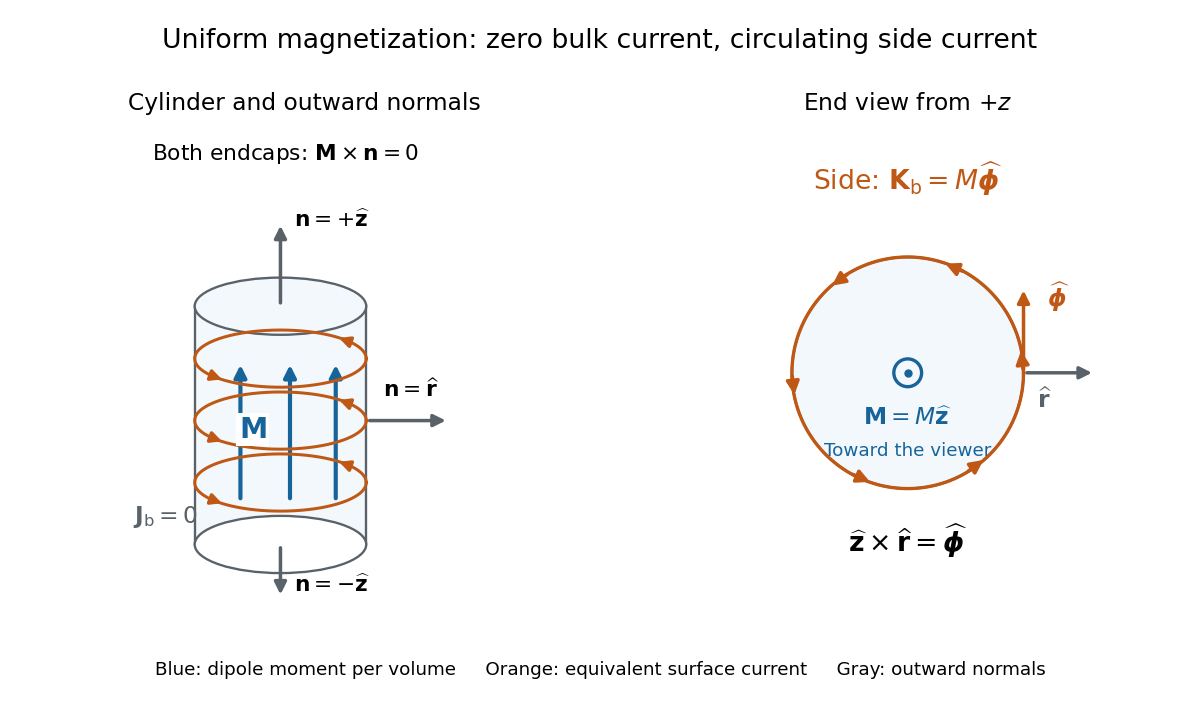
For an original example, let $M=800A/m$, $R=0.020\mathrm{m}$, and $L=0.10\mathrm{m}$. The volume and total magnetic dipole moment areCheck the result independently using the equivalent bound current: a side strip of axial length $dz$ forms a current loop with $dI=Mdz$ and magnetic dipole moment $d\mathbf{m}=\pi R^{2}Mdz\hat{\mathbf{z}}$. Its integral over $L$ gives the same $M\pi R^{2}L\hat{\mathbf{z}}$. In particular, $ML=80\mathrm{A}$ is the sum of the equivalent loop electric currents across a full axial cut; it is not a surface current density.

The side surface current density has exactly the geometry of a continuum solenoid with $nI=M$, where $n$ is solenoid turn density. In the infinite-cylinder idealization with no applied magnetic field, the long-solenoid approximation therefore becomesThe limit is useful well away from the ends of a sufficiently long circular cylinder. A finite circular cylinder instead has fringing magnetic field and a demagnetizing field. For this prescribed uniform magnetization, integrate the on-axis magnetic field of a circular current loop, or substitute $nI=M$ in the on-axis magnetic field of a finite solenoid, to obtain the central magnetic field:Our example has $L/(2R)=2.5$ and $B_z(0)/({\mu }_{0}M)=5/\sqrt{29}\approx 0.92848$, rather than unity. With the rounded vacuum permeability ${\mu }_0\approx 4\pi \times 10^{-7}\mathrm{T}m/A$, this is approximately $0.9334\mathrm{mT}$, compared with the infinite-cylinder value $1.0053\mathrm{mT}$. These are model calculations for a prescribed magnetization, not measured values or a solution for the self-consistent magnetization of an arbitrary material.