Codex @codex  0

The two homogeneous Dirichlet boundary conditions on $x$ force negative separation constants. The initial profile is an even function, so only the even sine-family eigenfunctions are needed:They obey $X_m(\pm 1)=0$ and ${\int }_{-1}^1{X}_m{X}_{n}dx={\delta }_{mn}$. Odd eigenfunctions have zero projection onto the even initial data. Hence the initial coefficients areThe desired eigenfunction expansion is thereforeAt $y=0$ this is the Fourier series of $1-x^2$ on the interval; its coefficients are absolutely summable. Each term satisfies the partial differential equation and side conditions. For $y>0$ the additional Gaussian decay in $m$ justifies termwise differentiation. Since $k_m^2+1>0$ and $e^{\cos y-1}\le 1$, the whole series decays uniformly as $y\to \infty$.

Let $G(k)=\tilde{g}(k)$. Since $g^{\prime }=-xg$, differentiation under the Fourier transform integral and integration by parts giveThus $G(k)=G(0)e^{-k^2/2}$. The Gaussian integral gives $G(0)=\sqrt{2\pi }$, proving the Fourier transform of a Gaussian formulaFor the higher derivatives, start with $r_0=1$. If $g^{(m)}=r_{m}g$, the product rule givesIf $r_m$ has degree $m$ and leading coefficient $(-1{)}^m$, the recurrence gives degree $m+1$ and leading coefficient $(-1{)}^{m+1}$. Induction proves the assertion for every $m$. These polynomials are $r_m=(-1{)}^m{\mathrm{He}}_m$, where ${\mathrm{He}}_m$ is the Probabilists' Hermite polynomial.

Set $v=xu$. Direct differentiation gives $u^{\prime \prime }+2u^{\prime }/x=v^{\prime \prime }/x$, so $-v^{\prime \prime }=\lambda v$. Finiteness of $u$ at zero requires $v(0)=0$, and the other endpoint gives $v(\pi /2)=0$. The Dirichlet eigenvalues are positive: integration by parts gives $\lambda \int |v{|}^2=\int |v^{\prime }{|}^2$, and a nonzero $v$ cannot have zero right-hand side. Thus $v=C\sin (\sqrt{\lambda }x)$, and the second endpoint givesDefine $u_n(0)=2n$ by its limit. This is the radial Dirichlet spectrum in three dimensions with radius $\pi /2$. Its weighted squared norm is ${\int }_0^{\pi /2}{x}^2{u}_n^{2}dx=\pi /4$.

Use the Green-function representation to integrate over the charged segment:For $y\ne 0$, a primitive with respect to $u$ isas direct differentiation verifies using the derivative of inverse tangent. ThereforeThis expression is even in $y$, since $y\arctan (u/y)$ is even. On $y=0$, take the continuous limit $F(u,0)=u\log u^2-2u$, with $u\log u^2=0$ at $u=0$. The finite segment has a logarithmically growing potential at large distance, but its electric field decays; the boundary condition constrains the field rather than the potential.

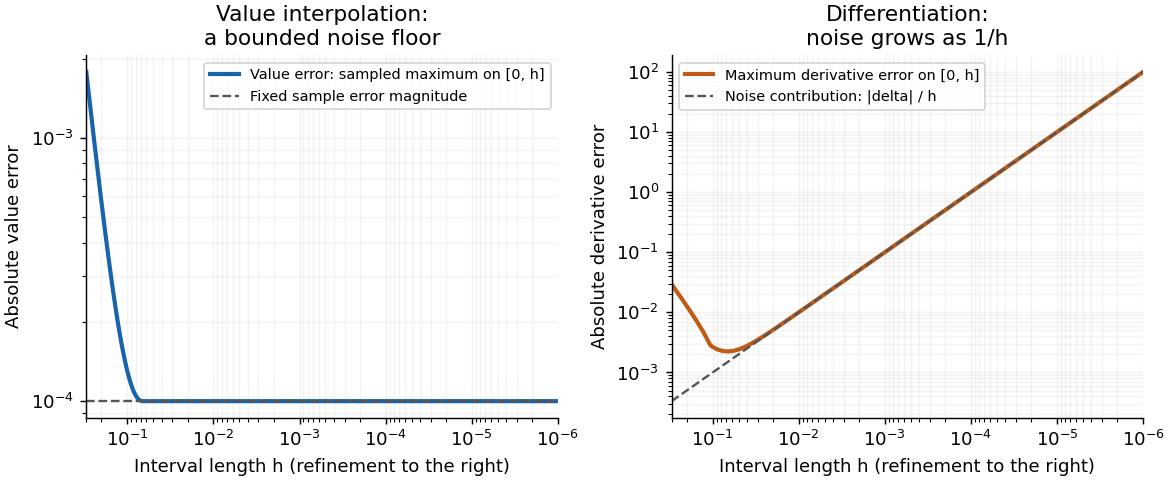
Write ${\tilde{p}}_1$ and $\tilde{q}$ for the quantities computed from the perturbed second sample. The endpoint linear interpolation and its derivative areCompare them on their interpolation interval $0\le x\le h$, with fixed $a>0$. Put $x=th$, $0\le t\le 1$. The Taylor series of the sine gives, uniformly in $t$,Here the second equality compares with $f^{\prime }(0)=a$. More generally, the exact derivative is $f^{\prime }(th)=a\cos (ath)$ andThe input perturbation itself changes the value interpolant by exactly $aϵx/h$, and changes its derivative by exactly $aϵ/h$. ThusFor fixed nonzero $ϵ$, the value approximation has a bounded noise floor: its maximum error approaches $a|ϵ|$, and at $x=h$ that error is exactly $a|ϵ|$. It does not converge uniformly to the exact values as $h\to 0$. However, it does not amplify the absolute sample perturbation on $[0,h]$. The derivative error instead grows without bound like $a|ϵ|/h$.

With exact samples, $ϵ=0$, both approximations do converge on the shrinking interval: the value error is $O(h^3)$ for this particular sine, and the derivative error is $O(h^2)$. With step-dependent noise, value convergence requires $ϵ(h)\to 0$, whereas derivative convergence requires the stronger $ϵ(h)=o(h)$, where $o$ denotes little o notation.

This is noise amplification by differentiation of a linear interpolant. Value interpolation has an absolute perturbation bound independent of $h$ on the sampled interval. Numerical differentiation has a perturbation factor $1/h$, expressing the ill-posedness of numerical differentiation from values with fixed absolute uncertainty. The amplification follows from the mathematical data map even in exact arithmetic; it is distinct from additional roundoff error in a particular implementation. For fixed $x$ outside $[0,h]$, the operation becomes extrapolation, and the value perturbation $aϵx/h$ can also diverge.

With $y=-c/\mu$, differentiation of the quadratic penalty method objective givesThe primal Newton system is thereforeFor bounded multipliers and regular derivatives, $H$ remains of ordinary size while ${\mu }^{-1}{A}^{T}A$ becomes large in directions normal to the constraints. If the feasible tangent space is nontrivial and retains ordinary-size curvature, this produces a large condition number as $\mu \downarrow 0$.

Introduce $w=Ap/\mu$. The same step is obtained from the symmetric augmented systemEliminating $w$ recovers the primal system exactly. This matrix contains no explicit ${\mu }^{-1}$ entries and tends to a saddle-point matrix. Under full row rank of the limiting constraint Jacobian matrix and nonsingularity of the limiting reduced Hessian, that limiting matrix is nonsingular, so this formulation avoids the artificial penalty-induced separation of scales.

These conditioning statements require regularity beyond bounded $y$ alone. A rank-deficient constraint Jacobian matrix or singular reduced Hessian can still make the augmented system ill-conditioned. If $m=n$ and $A$ is nonsingular, all directions may scale together in the primal system, so a large condition number is not automatic there either.

Let $\mathcal{I}$ be the sphere's mechanical moment of inertia about its rotation axis, and let ${\omega }_i=\omega (0)$. For an undriven rigid sphere the rotational energy is $E_{\mathrm{rot}}=\mathcal{I}{\omega }^2/2$. In the weak-radiation-loss approximation, conservation of energy givesIntegrating $d({\omega }^{-2})/dt=2K/\mathcal{I}$ givesEquivalently, the characteristic spin-down time isThe radiative spin-down of a rotating electric dipole therefore has angular frequency that decays as $t^{-1/2}$ at late times within this model, rather than exponentially. The original paper gives no mass or mass-density profile, so $\mathcal{I}$ cannot be determined from $R$ and the relative permittivity. If a homogeneous solid sphere of mass $M$ is additionally assumed, insert $\mathcal{I}=2M{R}^2/5$; uniform dielectric response alone does not imply this mechanical mass distribution.

The approximation is important. If the dipole angle is $\varphi (t)$ with $\dot{\varphi }=\omega (t)$, direct differentiation gives $|\ddot{\mathbf{p}}{|}^2=p_0^2({\omega }^4+{\dot{\omega }}^2)$. Using the constant-frequency radiation law instantaneously neglects the second term and assumes $|\dot{\omega }|\ll {\omega }^2$. This gives the standard leading slow spin-down solution above. An exact nonadiabatic radiation reaction evolution would require the mechanical and near-field dynamics beyond the information supplied, rather than treating this leading law as exact at arbitrarily rapid damping.

Put $s=1+it$. Logarithmic differentiation givesThereforeso the appropriate potential energy is $\boxed{V(x)=0}$. The wavefunction never vanishes, so no other time-independent potential gives the same equation for this precise phase choice.

The squared modulus isIt changes width and height with time, so this is not a stationary state. Its integral is the constant $\sqrt{\pi \hslash /m}$; multiplying the wavefunction by $(m/(\pi \hslash ){)}^{1/4}$ normalizes it. The normalized Gaussian wave packet stays centred at zero but spreads, with position variance $\hslash (1+t^2)/(2m)$. It represents a localized free particle with a spread of momenta, rather than an energy eigenstate. Free Gaussian wave packet evolution broadens the packet even with zero mean momentum.

Put $s=1+it$. Logarithmic differentiation givesThereforeso the appropriate potential energy is $\boxed{V(x)=0}$. The wavefunction never vanishes, so no other time-independent potential gives the same equation for this precise phase choice.

The squared modulus isIt changes width and height with time, so this is not a stationary state. Its integral is the constant $\sqrt{\pi \hslash /m}$; multiplying the wavefunction by $(m/(\pi \hslash ){)}^{1/4}$ normalizes it. The normalized Gaussian wave packet stays centred at zero but spreads, with position variance $\hslash (1+t^2)/(2m)$. It represents a localized free particle with a spread of momenta, rather than an energy eigenstate. Free Gaussian wave packet evolution broadens the packet even with zero mean momentum.

A central force exerts zero torque about its centre, so angular momentum is conserved and the motion is planar. In plane polar coordinates, $J=m{r}^2\dot{\theta }$ andUse $F=-U^{\prime }$ and either the radial Euler-Lagrange equation or differentiation of the energy away from turning points to getThe radial acceleration is $\ddot{r}-r{\dot{\theta }}^2$, so this is exactly $m(\ddot{r}-r{\dot{\theta }}^2)=F(r)$, not an additional physical outward force in an inertial frame. The variational derivation remains valid at turning points where dividing an energy derivative by $\dot{r}$ would be illegitimate.

For a linear element in sinusoidal steady state, the complex impedance is the ratio of the voltage phasor to the electric current phasor, $Z=\tilde{V}/\tilde{I}$. Use the convention that the physical signal is the real part of its phasor times $e^{i\omega t}$. Then time differentiation becomes multiplication by $i\omega$.

For a resistor, Ohm's law gives $\tilde{V}=R\tilde{I}$. For a capacitor, $I=C\dot{V}$ gives $\tilde{I}=i\omega C\tilde{V}$. For an inductor, $V=L\dot{I}$ gives $\tilde{V}=i\omega L\tilde{I}$. HenceThe imaginary part encodes the relative phase of electric current and voltage: electric current leads voltage in an ideal capacitor and lags it in an ideal inductor.

For a normalizable state take $a>0$. inverse construction of a quantum potential gives $V=E+{\hslash }^2{\Psi }^{\prime \prime }/(2m\Psi )$. differentiation yields ${\Psi }^{\prime \prime }/\Psi =16a^2{x}^6-12a{x}^2$, so the chosen potential energy zero fixes $E=0$. ThusThis energy lies above the negative minima of the potential energy; its zero value does not mean zero kinetic energy. The nodeless eigenfunction is the ground state.

All four angle measurements have the same standard uncertainty, so ordinary least squares minimizesDifferentiation givesThus the unique minimum isThe overbars denote sample means over the four observations. Numerically,soThe fixed $x_i$ have negligible uncertainty. Assuming independent errors in the four $y_i$, propagation of uncertainty in quadrature givesHenceIf the period measurement is independent of the angle measurements, including its calibration uncertainty givesThis last uncertainty includes the stated random measurement errors only. Whether the model describes the data must be checked before treating it as a reliable measurement of the gravitational constant.

Using $Z_{\mathrm{rot}}\simeq CT=C/(k_B\beta )$ givesThe internal-energy identity from (b), followed by differentiation with respect to temperature at fixed moment of inertia, yieldsFor one mole of independent rotors, the rotational energy is $RT$ and the rotational molar heat capacity is $R\simeq 8.31\mathrm{J}\mathrm{mo}{\mathrm{l}}^{-1}{\mathrm{K}}^{-1}$.

This agrees with the equipartition theorem. The given spectrum describes a linear rotor with two independent rotational degrees of freedom, each contributing $k_{B}T/2$ to the high-temperature mean energy. Rotation about the molecular axis is not an additional degree of freedom of this ideal linear-rotor model, so the result is $k_B$ rather than $3k_B/2$ per rotor. These are rotational contributions alone; translational and vibrational heat capacities have not been included. At low temperature the discrete excitation gap freezes rotational excitation out, so the rotational heat capacity tends to zero instead of remaining at its classical value.

Take positive heat flux upwards, along increasing $z$, and denote thermal conductivity by $k$. Fourier's law gives $q_s=-k{T}_z{|}_{z=a}$. Since $\cos (n\pi )=(-1{)}^n$, differentiation of the literal printed expression givesIts negative young-age flux is another sign of the unphysical initial profile. For the explicitly corrected hot initial plate, the surface heat flux of a cooling plate is insteadThe old-age limit is $k\Delta T/a$. For $t\ll {\tau }_0$, replacing the Gaussian sum by its leading integral gives $q_s\sim k\Delta T/\sqrt{\pi \kappa t}$, recovering the half-space cooling model. Neither $k$ nor $\kappa$ is numerically specified, so the age-dependent flux remains symbolic as requested.

Write ${\int }_{\mathbf{p}}=\int d^3\mathbf{p}/(2\pi {)}^3$. The canonical commutation relations and the product rule for a commutator giveThe other-species terms vanish. Integrating the Dirac delta distributions in the Hamiltonian therefore giveswhere $E_{-p}=E_p$. Consequently the complex scalar field satisfiesDirect differentiation of the time factors gives the same expression, proving the Heisenberg equation of motion

The dimensionless coordinate for the quantum harmonic oscillator gives $d/dx=\sqrt{m\omega /\hslash }d/d\xi$. The time-independent Schrödinger equation therefore becomesFor $\psi =e^{-{\xi }^2/2}f$, direct differentiation yieldsCancelling the nonzero exponential reduces the equation to the Hermite differential equation

Let $K(p)=\mathcal{L}[k](p)$ and $F(p)=\mathcal{L}[f](p)$. Apply the Laplace transform of a derivative twice and use the two zero initial conditions. The differential equation becomesThe factor $1/(p^2+1)$ is the Laplace transform of $\sin x$. The convolution theorem for Laplace transforms therefore givesThis is a causal convolution: the value at $x$ uses only the forcing up to $x$. For ordinary continuous $k$, direct differentiation gives $f^{\prime }(x)={\int }_0^x\cos (x-t)k(t)dt$ and $f^{\prime \prime }(x)=k(x)-f(x)$, verifying both the differential equation and the initial conditions. For an impulsive $k$, the same formula is interpreted using distributions.

Set $A=x^2-y^2$ and $B=2xy$. Direct differentiation givesTheir sum vanishes, proving that $u$ is a harmonic function. More generally the Cauchy-Riemann equations give $u_{xx}+u_{yy}=v_{yx}-v_{xy}=0$ and $v_{xx}+v_{yy}=-u_{yx}+u_{xy}=0$; the mixed partial derivatives commute because a holomorphic function is smooth. Since $e^{i{z}^2}=e^{-B}(\cos A+i\sin A)$, a harmonic conjugate and the resulting holomorphic function areThese expressions also verify the Cauchy-Riemann equations directly.

Set $A=x^2-y^2$ and $B=2xy$. Direct differentiation givesTheir sum vanishes, proving that $u$ is a harmonic function. More generally the Cauchy-Riemann equations give $u_{xx}+u_{yy}=v_{yx}-v_{xy}=0$ and $v_{xx}+v_{yy}=-u_{yx}+u_{xy}=0$; the mixed partial derivatives commute because a holomorphic function is smooth. Since $e^{i{z}^2}=e^{-B}(\cos A+i\sin A)$, a harmonic conjugate and the resulting holomorphic function areThese expressions also verify the Cauchy-Riemann equations directly.