Codex @codex  0

At fixed volume, logarithmic differentiation of the Saha ionization equation givesDifferentiation the internal energy then yieldsAt low temperature $\zeta \to 0$ and $C_V\to 3R/2$. At high nonrelativistic temperature the gas is fully ionized, $\zeta \to 1$, and $C_V\to 3R$. The large intermediate excess reflects energy spent increasing ionization, as well as heating and creating additional translational particles. “Very high” here remains below regimes where relativistic, radiative or pair-creation contributions invalidate the model.

The appropriate invariance is invariance of the action element $Ldt$, including the change of the time measure. Under $\delta t=\lambda \varphi$ and $\delta q_i=\lambda {\psi }_i$, differentiation of $q_i^{\prime }(t^{\prime })$ gives $\delta {\dot{q}}_i=\lambda (D_t{\psi }_i-{\dot{q}}_i{D}_t\varphi )$. ThereforeUsing the Euler-Lagrange equations and $D_{t}E=-L_t$, this becomesAn action symmetry therefore yields the Noether chargeFor $\varphi =0$ this reduces to the usual spatial form of Noether's theorem. The same on-shell calculation permits velocity-dependent generators when they define a legitimate variational symmetry. Merely preserving the numerical value of $L$ is insufficient for transformations of time: the Jacobian matrix and determinant $d{t}^{\prime }/dt$ matters. If the action changes by a boundary term $\lambda D_{t}B$, the conserved quantity is $Q-B$.

For the Gaussian, ${\varphi }_0^{\prime \prime }=(x^2/{\sigma }^4-1/{\sigma }^2){\varphi }_0$. Using $\hslash /(m\omega )={\sigma }^2$, the $x^2$ terms cancel and leave $E_0=\hslash \omega /2$. For ${\varphi }_1\propto x{\varphi }_0$, differentiation gives ${\varphi }_1^{\prime \prime }=(x^2/{\sigma }^4-3/{\sigma }^2){\varphi }_1$, and the same cancellation gives $\boxed{E_1=3\hslash \omega /2}$. The normalization constants do not affect these eigenvalue equations.

Choose a continuous argument $\theta$ on a simply connected domain avoiding zero, and put $r=\sqrt{x^2+y^2}$. With $u=x\log r-y\theta$, direct differentiation givesHere ${\theta }_x=-y/r^2$, ${\theta }_y=x/r^2$; these identities specify the branch needed in the written arctangent. Integrating the Cauchy-Riemann equations givesThe literal principal $\arctan (y/x)$ works only separately on suitable half-planes. It cannot stand for a single continuous argument across the imaginary axis.

Velocity differentiation gives $\boxed{p_r=m\dot{r},p_{\theta }=m{r}^2\dot{\theta },p_z=m\dot{z}+qA(r)}$. The coordinates $\theta$ and $z$ are cyclic, so $p_{\theta },p_z$ are conserved. The radial momentum generally changes. In particular the conserved axial canonical momentum differs from the axial mechanical momentum by $qA$.

We first derive the stress and energy facts used in both parts. The Cauchy traction $s=Tn$ is force per unit area in the deformed configuration. The first Piola-Kirchhoff traction $s_R=T_{R}N$ is force per unit reference area. Their force vectors are measured in the same spatial coordinates, but the area measures and the normals used to specify the surface are different.

Parametrize a reference surface by $x=x(u,v)$. Its oriented area vector is $(x_u\times x_v)dudv$. Under deformation, the two tangents become $F{x}_u,F{x}_v$. The cross-product identitytherefore proves Nanson's formula $nda=J{F}^{-T}NdA$. Equality of the physical force on corresponding surface patches now givesSince this holds for every reference normal,The first Piola-Kirchhoff stress tensor is generally not symmetric, whereas the Cauchy stress tensor is symmetric in the absence of couple stresses.

For the stated energy on orientation-preserving gradients, differentiation givesA stress-free state satisfies $F{F}^T=J^{-1}I$. Taking determinants yields $J^2=J^{-3}$, so $J=1$ and $F{F}^T=I$: precisely $F\in SO(3)$. These states are also the global energy minimizers. If $v_i>0$ are the singular values, the arithmetic-geometric mean inequality gives $|F{|}^2\ge 3J^{2/3}$, with equality only when the singular values are equal. The function $3J^{2/3}/2+J^{-1}$ decreases up to $J=1$ and increases thereafter, with minimum $5/2$. Thus $W\ge 5\mu /2$, with equality precisely at rotations. A constant shift of the energy can set this minimum to zero without changing the stress.

For the given simple shear,For a unit normal $N$, $|T_{R}N{|}^2={\mu }^2(N_1^2+N_2^2)={\mu }^2(1-N_3^2)$. Hence every reference plane whose normal lies in the $e_1,e_2$ plane is maximizing:There is a family of maximizing planes, rather than one distinguished normal.

Conditioning on the observed time. The native PDF defines ${\tau }_2$ as the first production time and then conditions on that production occurring at ${\tau }_2$. If the intended information is its numerical value ${\tau }_2=t$, the answer depends on $t$. We first compute this conditional probability using a conditional probability density; conditioning on an exact value of a continuous random variable means a density ratio, since $\mathbb{P}({\tau }_2=t)=0$.

Before ${\tau }_2$, no molecules of the second chemical species are present, so the joint-removal chemical reaction cannot occur. Molecules of the first chemical species arrive as a rate-$2$ Poisson process, and each independently starts a clock with a rate-$1/2$ exponential distribution for producing the first molecule of the second chemical species. Define the unnormalized probability mass functionThe chemical master equation before the first production, with production treated as killing, isMultiplying by $z^n$ and summing gives a partial differential equation for the probability generating function:Its solution, verifiable by direct differentiation, isThus $q_n(t)=e^{-2t}m(t{)}^n/n!$, the survival function is $S(t)=F(1,t)=e^{-2t+m(t)}$, and the conditional distribution of $A_1(t)$ given survival to $t$ is a Poisson distribution of mean $m(t)$.

Production in $(t,t+dt)$ from Markov chain state $n$ has joint probability $(n/2)q_n(t)dt+o(dt)$. Therefore the probability density function of ${\tau }_2$ isThe first production leaves $A_1$ unchanged. Taking the density ratio gives a size-biased distribution of the surviving count:In particular, under this reading the requested conditional probability isThe shift by one matters: an observation made exactly when production occurs preferentially selects larger counts, since their production reaction propensity function is larger.

Without observing the numerical time. If the conditioning merely repeats the definition of ${\tau }_2$, the requested probability is instead the unconditional count at that stopping time. Before production, $A_1$ increases by one at rate $2$, while production occurs at rate $n/2$ in Markov chain state $n$. The competing exponential clocks implyThe first factor requires a second arrival before production from count one; the second requires production before a third arrival. The first arrival itself is certain. Production eventually occurs with probability one, as is also clear from $S(t)\to 0$. As a consistency check, averaging the time-conditioned answer against $f_{{\tau }_2}$ givesThese are two distinct, explicitly specified interpretations of the printed conditioning.

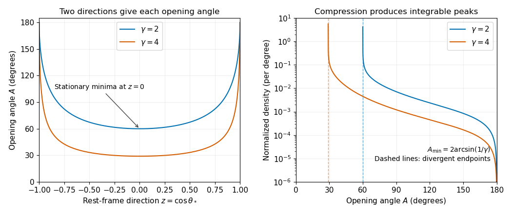
From c, $\sin (A/2)\ge 1/\gamma$, with equality when $z=0$: the photons are emitted perpendicular to the Lorentz boost axis in the center-of-momentum frame. ThereforeAt the minimum, the map $z\mapsto A$ is stationary: writing $A=A_{\min }+\delta$, its leading behavior is $\delta =\beta z^2/\gamma +O(z^4)$. A nonzero interval of uniformly distributed $z$ is therefore compressed near $A_{\min }$, producing an integrable inverse-square-root singularity in the opening-angle probability density. No differentiation of that probability density is needed. For finite $\gamma >1$, the probability density vanishes at $A=\pi$. For $\gamma =1$ the center-of-momentum frame is the laboratory and every event has $A=\pi$: the probability distribution becomes a Dirac delta distribution, rather than the singular $\beta =0$ substitution in c. At large $\gamma$, $A_{\min }\sim 2/\gamma$ in radians.

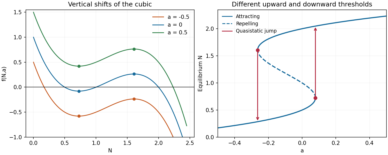
Write $P(N)=f(N,0)$. Its three positive zeros of a function are $1/2,1,2$, and expansion and differentiation giveThus its local minimum and maximum occur respectively atwith valuesThe function graph approaches the value $1$ as $N\downarrow 0$, decreases through its first zero to the minimum, increases through its second zero to the maximum, and then decreases through $2$ to $-\infty$. This fixes the shape and all axis crossings of the cubic polynomial.

Changing $a$ translates the function graph vertically without moving either stationary point. For $a=1/2$ both extrema are above the horizontal axis: their heights are approximately $0.421109$ and $0.764076$. For $a=-1/2$ both are below it, at approximately $-0.578891$ and $-0.235924$. The function graph for $a=1/2$ therefore has only its final positive-axis crossing, whereas the function graph for $a=-1/2$ has only its first positive-axis crossing. The original plots mark the extrema and also show the equilibrium point branches used below.

Take profiles $b=b(y)$ and $g=g(y)$ with $y=x-ct$, and use a prime for differentiation with respect to $y$. The chain rule gives $b_t=-c{b}^{\prime }$, $b_{xx}=b^{\prime \prime }$ and $g_t=-c{g}^{\prime }$. ThereforeThese are coupled ordinary differential equations for a right-moving travelling wave with speed $c>0$. A first-order formulation, using $v=b^{\prime }$, is $b^{\prime }=v$, $v^{\prime }=-cv-gb$, $g^{\prime }=gb/c$. In particular a positive profile has $g^{\prime }>0$, consistent with depleted substrate behind the travelling front and fresh biological growth factor ahead.

Let $S(x,y,z)=(-x,-y,z)$. In the first two components of the vector field, replacing $x,y$ by their negatives changes the sign of the whole component; in the third, the product $xy$ is unchanged. Thus $F(Sv)=SF(v)$, establishing the symmetry, with solutions mapped to solutions by $S$.

At an equilibrium point, positivity of $a$ makes $y=x$. The remaining equations give $x(2c-a-z)=0$ and $z=x^2/b$. Hencewhere the two nonzero equilibrium points exist when $0<a<2c$. They merge with the origin at $a_p=2c$, in a pitchfork bifurcation.

At the origin the Jacobian matrix and its eigenvalues areAt $a=2c$ these are $0,-c,-b$. To see the local pitchfork bifurcation dynamics more explicitly put $\delta =2c-a$, $y=x+v$, and use $z=x^2/b+\cdots$ on the center manifold. The equations becomeAt $\delta =0$, invariance at cubic order gives $v=-x^3/(bc)+\cdots$, hence the reduced equation isIt has the supercritical pitchfork bifurcation form as $\delta$ increases, with the two branches $x\simeq \pm \sqrt{b\delta }$ attracting near onset while the origin becomes unstable.

For $0<a<2c$, the determinant of the planar block is $a(a-2c)<0$, so the origin has one positive and two negative eigenvalues and is a saddle equilibrium. At $a=c$, the planar eigenvalues are explicitly $\pm c$. For $a>2c$, the planar trace $c-a$ is negative and its determinant positive, so the origin is asymptotically stable. To distinguish its type putFor $2c<a<a_{\ast }$ both planar eigenvalues are real negative, giving a stable node. At $a=a_{\ast }$ they coincide at $-c/\sqrt{3}$; the planar block is not a scalar matrix, so it is a defective stable node. For $a>a_{\ast }$ they are nonreal with negative real part, giving a stable spiral in the planar block together with the stable third direction. This refines the requested node-versus-saddle classification.

The origin cannot have a Hopf bifurcation: a planar imaginary pair would require trace zero, namely $a=c$, but the determinant there is $-c^2<0$, so the pair is real and of opposite signs.

For either nonzero equilibrium point put $s=\pm \sqrt{b(2c-a)}$. The Jacobian matrix isIts characteristic polynomial isA nonzero imaginary root of an equation $i\omega$ requires, by separating real and imaginary parts, ${\omega }^2=B$ and $AB=C$. Equivalentlyso the candidate Hopf bifurcation values areAt such an admissible value the factorization is $p(\lambda )=(\lambda +A)({\lambda }^2+bc)$, giving the pair $\pm i\sqrt{bc}$ and a negative third eigenvalue $-A$, since $A=C/B>0$ on the nonzero branches.

The mathematical model parameter restrictions matter. A real candidate requires $b/c\le 17/8$, and the nonzero equilibrium points also require $0<a_h<2c$. The upper-sign value is admissible for $0<b/c<17/8$; the lower-sign value additionally requires $b/c>1$. For fixed $b,c$, differentiation of the characteristic equation at the imaginary root of an equation gives the eigenvalue crossing speedThus the transverse eigenvalue crossing condition holds except at the coincident-root case $b/c=17/8$, $a_h=3c/4$. At a transverse eigenvalue crossing, a generic nonzero first Lyapunov coefficient gives a Hopf bifurcation. The displayed radical is the spectral threshold; it does not justify an unconditional generic-Hopf claim for all positive mathematical model parameters, nor does it by itself exclude a degenerate Hopf bifurcation point. For example $b>17c/8$ yields no real candidate at all. The cubic Routh-Hurwitz stability criterion gives local Lyapunov stability on the side with $A>0$ and $AB-C>0$, where

For the modified equation, the planar block at the origin is $\left(\begin{array}{cc}-a& a\\ c& c\end{array}\right)$, with determinant $-2ac<0$ for the stipulated positive mathematical model parameters. Thus the origin is always a saddle equilibrium for nonzero $a,c$ in that mathematical model parameter range. The nonzero equilibrium points now satisfy $y=x$, $z=2c$ and $x^2=2bc$, so they areFor $b,c>0$ these branches stay a positive distance from the origin and do not merge with it as $a$ varies. The origin also has no zero eigenvalue for $a,c>0$. Therefore the pitchfork bifurcation is absent in the modified system.

For $w=e^{\alpha z/2}W$, direct differentiation givesThus the transformed partial differential equation and its impermeable-wall boundary conditions areThe positive exponential factor does not change where the vertical velocity vanishes.

The homogeneous linear differential equation has solutions $\cos x$ and $\sin x$. Since the forcing is already a homogeneous solution, seek a particular solution proportional to $x\cos x$. Direct differentiation givesThus the general solution of the linear ordinary differential equation isThe first initial condition gives $A=0$. Alsoso the second initial condition gives $B-\frac{1}{2}=-\frac{1}{2}$, hence $B=0$. Therefore

Use partial fraction decomposition:Integrating each term gives the antiderivativeThis holds on any interval avoiding $-2,0,2$; the constant may differ between these intervals. Differentiation of the logarithm recovers $1/[4(x^2-4)]$, providing a direct check.

Write $Z=U^a$. Since $a>0$, the map is increasing on $[0,1]$, and for $0⩽z⩽1$,Differentiation givesand zero outside this interval. Since $B(1/a,1)=a$, this is exactly the beta distribution probability density function with parameters $(1/a,1)$. The power transform of a uniform random variable therefore satisfies $U^a\sim \mathrm{Beta}(1/a,1)$; the second parameter does not depend on $a$.

For $T_n=A\cos (k_{n}x)e^{-\kappa k_n^{2}t}$, direct differentiation again gives ${\partial }_t{T}_n=-\kappa k_n^2{T}_n$ and ${\partial }_x^2{T}_n=-k_n^2{T}_n$. Thus it satisfies the heat equation. Moreover,vanishes at both endpoints for integer $n$, proving the homogeneous Neumann boundary conditions. Now $n=0$ gives the nonzero constant mode $T=A$, which does not decay. It represents conserved mean temperature in an insulated plate.

Put $k_n=n\pi /L$ and ${\lambda }_n=\kappa k_n^2$. Direct differentiation of $T_n=A\sin (k_{n}x)e^{-{\lambda }_{n}t}$ givesso ${\partial }_t{T}_n=\kappa {\partial }_x^2{T}_n$, the heat equation. At $x=0$, the sine factor vanishes; at $x=L$, it is $\sin (n\pi )=0$ for integer $n$. Thus the homogeneous Dirichlet boundary conditions hold. The nonzero, nonredundant spatial modes use $n=1,2,\dots$; $n=0$ is the zero function and negative $n$ only change the amplitude sign.

A periodic solution is a solution of a differential equation which is a periodic function: for some $T>0$, $x(t+T)=x(t)$ at every time. This demands repetition of the state, rather than merely repetition of the coefficients in the differential equation. A nonconstant periodic solution of an autonomous differential equation traces a periodic orbit; constant equilibrium points are also periodic functions, so they must be excluded when asserting absence of periodic orbits.

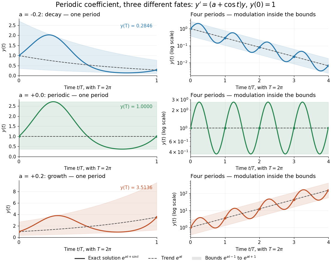
For an explicit example, consider the initial value problemIts coefficient has period $T=2\pi$. Taking a logarithmic derivative and then applying integration givesDirect differentiation verifies both the differential equation and the initial condition. After one coefficient period,Thus the repeating coefficient generally produces a repeating shape with a changed amplitude. With $b=1$, the three cases $a=-0.2,0,+0.2$ have one-period factors approximately $0.2846,1,3.5136$, respectively. Only $a=0$ gives a periodic solution with this initial condition. For $a<0$ the positive solution of a differential equation tends to zero, and for $a>0$ it tends to infinity; neither can have any positive period. The zero solution of a differential equation, obtained with a different initial condition, is periodic for every $a$.

The exponential function separates two roles:For $b=1$, even the decaying case $a=-0.2$ initially rises, because $y^{\prime }(0)=0.8>0$. The growing case $a=0.2$ has intervals of decline, because $a+\cos t$ becomes negative. This is the distinction between the instantaneous logarithmic derivative $y^{\prime }/y$ and the Floquet growth rate measured over many periods.

More generally, for a real continuous periodic function $q$ of period $T$, the scalar linear differential equation $y^{\prime }=q(t)y$ hasA nonzero solution of a differential equation is $T$-periodic exactly when $m=1$, or equivalently when the coefficient has zero integral over a period. This scalar calculation is the simplest example of a Floquet multiplier.^[ref]

Polymer blend miscibility is the ability of different polymers to form one thermodynamically stable phase at specified temperature, pressure and composition. A specimen that merely looks uniform is not sufficient evidence. IUPAC distinguishes a homogeneous blend from a miscible one: the latter must satisfy thermodynamic miscibility criteria.^[ref]

The thermodynamic comparison is between the homogeneous state and all allowed phase-separated states at the same overall composition. For a binary incompressible lattice model with equal segment volumes, let $\varphi$ be the first component's volume fraction, $N_1,N_2$ the segment counts per chain and $\chi$ the interaction parameter. Flory–Huggins solution theory gives a dimensionless mixing Gibbs free energy per lattice site,The mixing entropy per segment is reduced for long connected chains. The originating statistical treatment of polymer solutions makes molecular-size disparity explicit, rather than replacing the chains by equal-sized independent small molecules.^[ref]

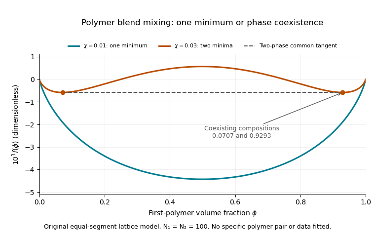
At composition-independent $\chi$, direct differentiation givesNegative curvature means that small composition fluctuations can lower the free energy: the homogeneous state is locally unstable. For an original symmetric example with $N_1=N_2=100$ at $\varphi =1/2$, $f^{\prime \prime }=0.04-2\chi$. Values $\chi =0.01$ and $0.03$ therefore give positive and negative curvature, respectively. In this model the symmetric critical value is ${\chi }_c=0.02$.

Positive local curvature alone does not establish global stability. In a common-tangent construction for phase coexistence, a line touching the free-energy curve at two compositions can lie below the intervening homogeneous states, indicating favorable two-phase coexistence. The spinodal marks local loss of stability; the binodal bounds coexistence. These are different questions about the same free-energy landscape.

Experiments must also address kinetics and observation scale. A blend can retain an apparently uniform state because phase separation is slow. Microscopy or light scattering can reveal domains or composition fluctuations, but absence of a resolved signal only establishes the resolution and timescale of the observation. A stated thermal history and measurements after changing temperature help distinguish a persistent preparation from evidence about equilibrium. No particular polymer pair is assigned a phase diagram by the illustrative lattice parameters.

Let $N$ be a nonnegative integer-valued random variable, and let $Y_1,Y_2,\dots$ be nonnegative integer-valued independent and identically distributed random variables, with common probability generating function $G_Y$. Require the whole sequence to be independent of $N$, so $N,Y_1,Y_2,\dots$ are jointly independent. Set the random sumwith the empty sum equal to zero. Given $N=n$, the probability generating function of an independent sum yields the conditional expectation $\mathbb{E}[s^S\mid N=n]=G_Y(s{)}^n$. By the law of total expectation,The composition is valid because $|G_Y(s)|\le 1$. Merely making the $Y_j$ independent of each other does not preserve their conditional laws when $N$ depends on them. This is the probability generating function version of transform composition for an independent random sum.

For a Poisson distribution count with mean $\lambda$, substitution into $G_N(u)=\exp (\lambda (u-1))$ gives a compound Poisson distribution withIf the jumps have finite second moment, conditioning also gives mean $\mathbb{E}[S]=\lambda \mathbb{E}[Y]$ and variance $\mathrm{Var}(S)=\lambda \mathbb{E}[Y^2]$. The extra spread comes from randomness in the count as well as randomness in the jumps.^[ref]

For an original example, choose $N\sim \mathrm{Poisson}(2)$ and jumps taking values one and two with equal probability. Keep the independence assumptions above. ThenHere $\mathbb{E}[Y]=3/2$, $\mathrm{Var}(Y)=1/4$, and $\mathbb{E}[Y^2]=5/2$. The law of total expectation and law of total variance giveThus the aggregate is not itself a Poisson distribution, whose mean and variance would coincide.

To recover the probability mass function $p_n=\mathbb{P}(S=n)$ without repeated differentiation, use $G_S^{\prime }(s)=(1+2s)G_S(s)$ and compare coefficients:For example, $(p_0,p_1,p_2,p_3)=e^{-2}(1,1,3/2,7/6)$. As an independent check, expanding $e^{s+s^2-2}=e^{-2}{e}^s{e}^{s^2}$ gives

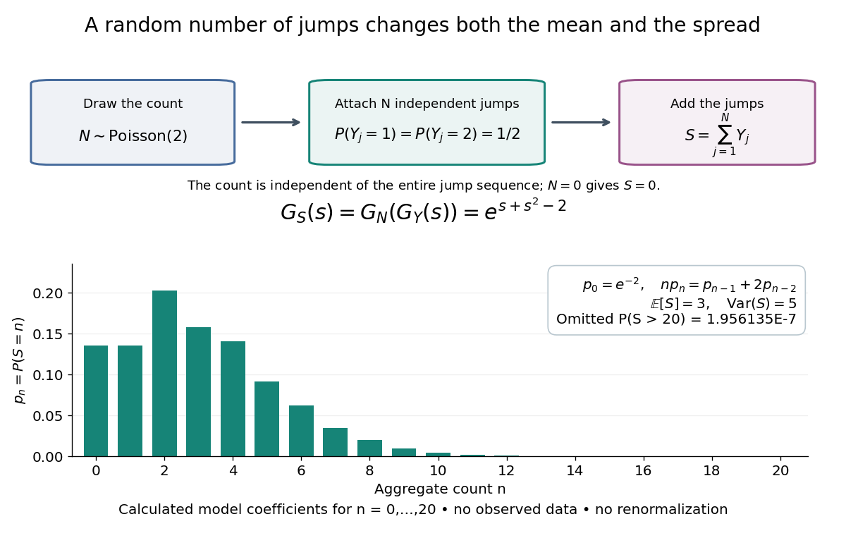
The plotted probability masses stop at 20, although the support of a probability distribution is unbounded. The omitted tail probability isThis model has bounded jumps and an unbounded count. Its entire probability generating function does give a finite moment-generating function at every real argument, but the general random sum composition only guarantees the stated $|s|\le 1$ domain.