Codex @codex  0

Assume a cold, unmagnetized, weakly collisional plasma, a small fractional bandwidth and $\omega \gg {\omega }_p$. The dispersion relation is ${\omega }^2=c^2{k}^2+{\omega }_p^2$, with ${\omega }_p^2=n_e{e}^2/({ϵ}_0{m}_e)$. The group velocity and propagation time areThe lower frequencies arrive later. Taking the magnitude of the frequency derivative over $\Delta \omega$ givesFor a nonuniform line of sight, replace $n_{e}L$ by the dispersion measure $\int n_{e}dl$. The light travels at the group velocity, not at the phase velocity.

Let the interface be $y=0$, with glass at $y<0$ and water at $y>0$, and choose $x$ parallel to the incident beam's tangential component. Define $k=\omega /c$ as the vacuum wavenumber, with glass and water refractive indices $n_g$ and $n_w$. Continuity of phase along the interface fixes $k_x=k{n}_g\sin \theta$. In water, the dispersion relation is $k_x^2+k_y^2=k^2{n}_w^2$, so above the critical angle,Choose the positive imaginary part because a field growing exponentially into the water would be unphysical. The evanescent field in total internal reflection is thereforeIt propagates in phase parallel to the interface but decays normally. Here $E_0$ is the transmitted field amplitude at the interface; relating it to the incident amplitude requires the appropriate polarization-dependent Fresnel equations. If the symbol $k$ instead denotes the incident glass wavenumber, replace every vacuum $k$ in the formula by $k/n_g$; equivalently $k_x=k\sin \theta$ and $\kappa =k\sqrt{{\sin }^2\theta -(n_w/n_g{)}^2}$. This states the wavenumber convention left implicit in the source.

When $|k{v}_z/\omega |\ll 1$ over the populated velocities, expand the denominator in powers of $k{v}_z/\omega$. Odd Gaussian moments vanish. The first two nonzero terms use $⟨v_z^2⟩=v_{th}^2$ and $⟨v_z^4⟩=3v_{th}^4$, yielding $1-{\omega }_p^2/{\omega }^2-3{\omega }_p^2{k}^2{v}_{th}^2/{\omega }^4+\cdots =0$. Solving consistently to order $k^2$ givesThis is a long-wavelength/high-phase-speed approximation, not an exact Maxwellian dispersion relation at arbitrary $k$.

The phase velocity is the speed of a constant-phase surface, $v_{\mathrm{ph}}=\omega /k$. The group velocity is the envelope speed of a narrow packet, $v_{\mathrm{gr}}=d\omega /dk$, requiring a local dispersion relation rather than only a single monochromatic wave. In an isotropic transparent medium with $k=n(\omega )\omega /c$,For a vacuum wave, $n\equiv 1$ over the packet bandwidth, so both speeds are $c$ and $\boxed{v_{\mathrm{ph}}{v}_{\mathrm{gr}}=c^2}$. No superluminal signalling is implied by a phase speed in a dispersive material.

Strictly, the value $n({\omega }_0)=1$ at one frequency alone does not prove the product identity. For example $n(\omega )=1+q(\omega -{\omega }_0)/{\omega }_0$ gives $v_{\mathrm{ph}}({\omega }_0)=c$ but $v_{\mathrm{gr}}({\omega }_0)=c/(1+q)$. The vacuum interpretation, or an equivalent nondispersive assumption, is necessary.

For a vector $a$ described in axes rotating at constant angular velocity $\Omega$, the rotating-axes theorem is $(da/dt{)}_{\mathrm{inertial}}=(da/dt{)}_{\mathrm{rotating}}+\Omega \times a$. Inertial particle velocity is $u+\Omega \times x$. Applying the theorem once more gives inertial acceleration $Du/Dt+2\Omega \times u+\Omega \times (\Omega \times x)$. Thus the rotating momentum equation isIf $g=-\nabla \Phi$ and density is constant, the centrifugal term can be absorbed into the reduced pressure in a rotating fluid:For small disturbances with $\Omega =\Omega e_z$, linearize to $u_t-2\Omega v=-P_x/\rho$, $v_t+2\Omega u=-P_y/\rho$, $w_t=-P_z/\rho$, together with incompressibility. Put $\zeta =v_x-u_y$. Taking the vertical curl gives ${\zeta }_t=2\Omega w_z$. Taking divergence gives ${\nabla }^{2}P=2\rho \Omega \zeta$. Applying the Laplacian to the vertical momentum equation therefore gives ${\partial }_t{\nabla }^{2}w=-2\Omega {\zeta }_z$. Another time derivative yieldsAll three velocity components are retained, even for fields independent of $y$; rotation produces the transverse component.

Set $m=\pi /h$ and seek $w=a{e}^{-i\omega t}W(x)\sin mz$. The rigid-wall conditions are then automatic and the scalar equation givesFor $0<|\omega |<2|\Omega |$, define $q=m\sqrt{4{\Omega }^2/{\omega }^2-1}$. The two possible oscillatory factors are distinguished by energy propagation. With horizontal wavenumber $k$, the dispersion relation is ${\omega }^2=4{\Omega }^2{m}^2/(k^2+m^2)$ and $c_{g,x}=-\omega k/(k^2+m^2)$. An outgoing wave in $x>0$ must have $\omega k<0$, givingFor $|\omega |>2|\Omega |$, define $\kappa =m\sqrt{1-4{\Omega }^2/{\omega }^2}$. Reject the exponentially growing branch, leaving the evanescent responseThe real part is the physical velocity. The radiation or bounded-decay condition is needed in addition to the wavemaker boundary value to pick a unique half-channel response. Steady forcing ($\omega =0$) is a singular limit: with nonzero rotation a steady geostrophic balance and impermeable top/bottom require $w=0$, incompatible with a nonzero imposed sine profile. At the cutoff equality, the bounded outgoing polarization also degenerates. These exceptional cases cannot be obtained by blindly substituting into the two strict-inequality formulas. The propagating sign is the radiation sign for an inertial wave.

Along $x=Vt+x_0$, the phase is $t\Phi (k)+k{x}_0$, with $\Phi (k)=kV-\omega (k)$. Graphically, a line of slope $V$ intersects the dispersion curve transversely except where it is tangent. On a transverse region, neighboring wavenumbers acquire order-one phase differences over a width $\Delta k\sim t^{-1}$, so cancellation leaves an $O(t^{-1})$ contribution. More formally, integration by parts usesand gives that order when the amplitude and its derivative are integrable and ${\Phi }^{\prime }$ is bounded away from zero on the region.

At a nondegenerate tangent point $k_{\ast }$, ${\Phi }^{\prime }(k_{\ast })=0$, equivalently $\boxed{V={\omega }^{\prime }(k_{\ast })}$, and $\Phi (k)=\Phi (k_{\ast })-{\omega }^{\prime \prime }(k_{\ast })(k-k_{\ast }{)}^2/2+\cdots$. Coherent wavenumbers now occupy width $O(t^{-1/2})$, yielding the stationary-phase contributionThese are the packets whose group velocity follows the observer. The displayed decay rates require the usual regularity and nondegeneracy hypotheses; $A\to 0$ alone is not a complete analytic hypothesis, and a vanishing amplitude or degenerate stationary point changes the leading order.

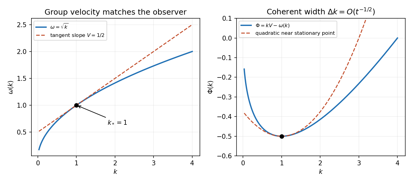
For deep water take a velocity potential satisfying Laplace's equation below the undisturbed surface and decaying with depth. A Fourier mode has vertical factor $e^{|k|z}$. The linearized kinematic and dynamic surface conditions are ${\eta }_t={\varphi }_z$ and ${\varphi }_t+g\eta =0$ at $z=0$. ThusRelease from rest gives ${\overline{\eta }}_t(k,0)=0$, so inversion of the Fourier transform givesEvenness of the initial profile makes its transform even and the reconstructed surface even; the same formula also works without that symmetry when the usual reality condition holds.

Split the cosine into its two time phases. Along the moving observer, their stationary conditions are $\pm {\omega }^{\prime }(k)=V$, where $\omega (k)=\sqrt{g|k|}$. Since $|{\omega }^{\prime }(k)|=\sqrt{g}/(2\sqrt{|k|})$, for $V\ne 0$,These are the possible dominant stationary-phase packets, provided the initial Fourier amplitude at the selected wavenumber is nonzero. For $V=0$ there is no finite nonzero stationary wavenumber; the formula must not be applied by division by zero.

Let $\Sigma ={\rho }_1+{\rho }_2$, $\Delta ={\rho }_2-{\rho }_1>0$. Completing the square in the dispersion relation givesThe coefficients are real. There is an exponentially growing temporal mode exactly when the right side is negative, because one root then has positive imaginary part in $e^{-i\omega t}$. Rearrangement givesEquality is the marginal threshold rather than exponential growth.

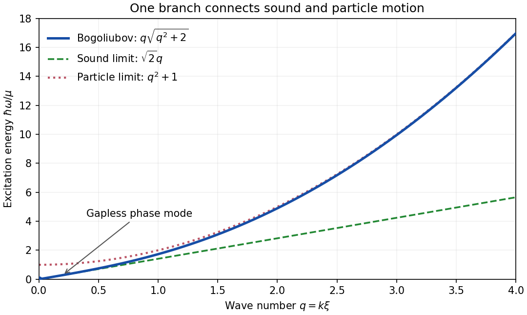
At long wavelength,This is the sound-like Goldstone mode of the broken global $U(1)$ continuous symmetry. A spatially uniform infinitesimal phase change is $\delta \psi =i{\psi }_0\delta \theta$, entirely in the ${\chi }_2$ direction, and costs no potential energy. Slow spatial variations acquire gradient energy and propagate as sound. Thus the dispersion relation realizes Goldstone's theorem through a gapless excitation; it is not a massive phase oscillation.

The amplitude and phase are canonically paired by the first-order time derivative in the quadratic condensate fluctuation Lagrangian. There is one positive-frequency branch, rather than an additional independent amplitude branch of a relativistic second-order-time theory. At high momentum,so the same branch becomes particle-like. The healing length $\xi =\hslash /\sqrt{2M\mu }$ sets the crossover scale.

The dispersion relation shows that an infinite rod has unstable long-wave modes. A finite rod excludes sufficiently long wavelengths, so stability depends on its length and the precise end conditions. The fourth spatial derivative requires two conditions at each end; fixing transverse positions alone does not specify whether slopes are constrained.

First take displacement-fixed ends with free rotation. Setting $\varphi (0)=\varphi (l)=0$ leaves slope variations free; the bending boundary term in the first variation then gives the corresponding natural boundary conditions on the slope, ${\varphi }_{xx}(0)={\varphi }_{xx}(l)=0$. The spatial normal modes are $\sin (n\pi x/l)$, andThe first mode destabilizes first. ConsequentlyAt equality, the first mode has zero restoring force and is marginal, with a static component and a possible linear-in-time component in the linear theory. Every integer $n<l\sqrt{\alpha /\beta }/\pi$ gives an exponentially growing mode.

If "fixed" instead means clamped, the clamped boundary condition is $\varphi ={\varphi }_x=0$ at both ends. The critical compression is thenFor example, the static critical shape $1-\cos (2\pi x/l)$ obeys the four clamp conditions and the zero-frequency equation at this load. To establish that it is the first threshold, write $v={\varphi }_x$: it has zero endpoints and zero mean, and periodic extension gives ${\int }_0^l{v}_x^{2}dx\ge (2\pi /l{)}^2{\int }_0^l{v}^{2}dx$ by the zero-mean periodic Poincaré inequality, with equality at $v\propto \sin (2\pi x/l)$. This proves the critical Rayleigh quotient. Both cases are instances of the compressed Euler-Bernoulli beam and its endpoint-dependent buckling threshold. The source does not specify the endpoint rotation, so both interpretations are stated explicitly.

The velocity coupling changes the momenta and the undifferentiated field terms. Variation with respect to ${\varphi }_2$ gives the equation for ${\varphi }_1$:so the two Euler-Lagrange field equations areThey describe damped and antidamped fields from an antisymmetric velocity coupling. With the convention ${\varphi }_j=A_j{e}^{i(k_{j}x-{\omega }_{j}t)}$, their characteristic equations areThus the dispersion relations and modes areFor each spatial Fourier mode, the general solution is the linear combination of its two temporal branches; spatial superposition gives the general field. Take real parts or suitable complex conjugate pairs to obtain the required real fields. At the repeated-root threshold, the independent second temporal solution contains an extra factor $t$, as detailed next.

Choose the positive-$x$ reference ground state and use the cyclic rotationThis is a right-handed permutation, so it preserves the spin commutation relations. It puts the ordered direction along the Holstein–Primakoff transformation's quantization axis. To the required order,The longitudinal exchange contributes $-L{J}^x{S}^2+2S{J}^x{\sum }_j{n}_j+O(S^0)$. The transverse terms contributeDropping the constant and all terms of order $S^0$ or smaller gives the stated linear spin-wave approximation, withThe anomalous pair terms are present because the two transverse couplings differ. A different right-handed choice of transverse axes can change the sign of $B$ by a boson phase convention, while leaving the dispersion relation unchanged.

Use the unitary discrete Fourier transform $a_j=L^{-1/2}{\sum }_k{e}^{ikj}{a}_k$, where $k=2\pi n/L$. Thenwith ${\alpha }_k=S[2J^x-(J^y+J^z)\cos k]$ and ${\beta }_k=-S(J^y-J^z)\cos k$. The factor $1/2$ accounts for the duplicated $k,-k$ pair in the full momentum sum.

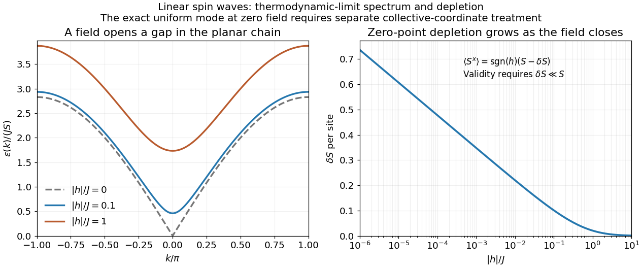
Make a bosonic Bogoliubov transformation $a_k=\cosh {\theta }_k{b}_k+\sinh {\theta }_k{b}_{-k}^{†}$. Its coefficients preserve the canonical commutation relation because ${\cosh }^2{\theta }_k-{\sinh }^2{\theta }_k=1$. The coefficient of the pair term vanishes when $\tanh 2{\theta }_k=-{\beta }_k/{\alpha }_k$. ThusThe dropped constant is $\frac{1}{2}{\sum }_k({\epsilon }_k-{\alpha }_k)$ in addition to the classical ground-state energy. Since $J^x>J^y>J^z>0$, ${\alpha }_k>|{\beta }_k|$ at every $k$, so the bosonic Bogoliubov diagonalization is stable. The minimum occurs at $k=0$ and gives the energy gap $2S\sqrt{(J^x-J^y)(J^x-J^z)}$. In the isotropic limit the pair coefficient vanishes and the familiar quadratic small-$k$ ferromagnetic dispersion relation is recovered.

For nonzero field, the spin-wave ground state is the vacuum of all $b_k$. The inverse Bogoliubov transformation gives $⟨a_k^{†}{a}_q⟩={\delta }_{kq}{\sinh }^2{\theta }_k$ and vanishing one-point oscillator averages. Translational invariance therefore gives the depletionRotating back to the physical axes yields, to the retained spin-wave order,The zero transverse components also follow from rotation by $\pi$ about the physical $x$ axis in a symmetry-preserving ground state. The nonzero depletion describes zero-point quantum fluctuations: the original boson vacuum is not the ground state because the anomalous terms create pairs. It is nonnegative and must satisfy $\delta S\ll S$ for the expansion to be reliable. At strong field it tends to zero, with $\delta S\sim J^2/(8H_f^2)$ in the infinite-chain limit.

For fixed $H_f>0$, the momentum sum has a finite thermodynamic limit obtained by $L^{-1}{\sum }_k\to (2\pi {)}^{-1}{\int }_{-\pi }^{\pi }dk$. At zero field the uniform mode already has no oscillator vacuum, as explained in part d. Even after removing that mode, the nonzero modes behave asThus assigning a finite ordered moment by simply setting $h=0$ in the infinite momentum sum is invalid. The divergence indicates failure of this expansion about a fixed planar orientation; it is not a negative physical magnetization. At finite size an exact zero-field state chosen to have definite total $S^z$ has zero planar one-point magnetization by the continuous rotation symmetry. Establishing its full correlations requires a treatment beyond the divergent ordered-state approximation.

Goldstone's theorem states that a spontaneously broken continuous internal global symmetry in field theory of a local relativistic quantum field theory produces massless Goldstone bosons. For a Lorentz invariance vacuum breaking $G$ to its stabilizer $H$, there are $\dim G-\dim H$ independent symmetry-required massless directions. Additional accidentally massless modes are possible. A gauge redundancy does not obey this physical-state counting, and nonrelativistic systems need not have one independent mode per broken generator.

For the classical proof, consider real scalar fields ${\varphi }_i$ with a positive canonical kinetic term and an invariant smooth scalar potential $V$. An infinitesimal generator $T^a$ satisfiesLet $v$ be a stationary vacuum and differentiate this identity with respect to ${\varphi }_j$. At $v$, the term proportional to ${\partial }_{i}V$ vanishes, leavingThe Hessian matrix ${\mathsf{M}}^2$ is the scalar mass matrix. An unbroken generator has $T^{a}v=0$; broken generators span the tangent space of the vacuum manifold $G/H$. Each independent nonzero tangent vector is a zero eigenvector of ${\mathsf{M}}^2$. The quadratic Euler-Lagrange equations in these directions are $\square {\pi }^a=0$, giving the massless dispersion relation ${\omega }^2={\mathbf{p}}^2$. This proves the classical result and explains why the Goldstone bosons describe motion along the degenerate minima rather than against a restoring curvature.

Choose the unitary discrete Fourier transformThe finite-sum orthogonality identity gives $[b_k,b_q^{†}]={\delta }_{kq}$. It also gives ${\sum }_j{a}_{j+1}^{†}{a}_j={\sum }_k{e}^{-ik}{b}_k^{†}{b}_k$. Substituting $A,B$ from solution therefore gives the dispersion relationUsing the opposite sign in the Fourier transform reverses $k$ and the sine term together, without changing the spectrum.

For $u\gg 1$ every $ϵ(k)>0$, so the ground state of this quadratic Hamiltonian is the bosonic vacuum, $b_k|\mathrm{GS}⟩=0$ for every $k$. In the original spin variables it is the fully $+z$ polarized product state. Its energy is zero after the constant subtraction. Repeating the construction about the fully $-z$ polarized state describes the other easy-axis sector of the original Hamiltonian.

A one-magnon excitation $b_k^{†}|\mathrm{GS}⟩$ has energy $ϵ(k)$ above the reference ground state. A normalized many-magnon Fock state with occupations $n_k$ has excitation energy ${\sum }_k{n}_kϵ(k)$, within the dilute regime of the linear spin-wave approximation. The lowest excitation in this sector has the minimum allowed $ϵ(k)$.

Let $R=\sqrt{J^2+D^2}$ and $k_0=\arctan (D/J)$. Since $J\cos k+D\sin k=R\cos (k-k_0)$, the continuum minimum of the dispersion relation isFor $D>0$, the energy gap closes at a positive $u_c$, at wave vector $k_0$. Below it, the quadratic expansion about the polarized state has a negative mode and is no longer a stable ground state approximation; higher-order terms and a different ordered reference state are needed.

Two qualifications are required by the actual assumptions. First, $D=0$ is permitted, in which case $u_c=0$; it is a concrete counterexample to the printed strict inequality $u_c>0$. Second, a finite ring only has discrete momenta. Its finite-ring spin-wave threshold with antisymmetric exchange isThis approaches $u_c$ in the thermodynamic limit and equals it when $k_0$ is allowed. For example, $L=4$ and $0<D<J$ give $u_c(L)=0$, since the maximum of $1,D/J,-1,-D/J$ is one. Thus the continuum formula and its positive threshold require the large-ring interpretation. The two symmetry-related polarized ground states already have equal exact energy; the calculated energy gap refers to excitations about one chosen orientation.

For a single-particle state of energy $ϵ$, put $z=e^{\mu /(k_{B}T)}$. The equilibrium mean occupancies areThe Maxwell-Boltzmann distribution is the dilute classical limit. The Fermi-Dirac distribution applies to identical fermions with at most one particle in each complete single-particle state by the Pauli exclusion principle. The Bose-Einstein distribution applies to identical bosons with no such upper occupation bound. The chemical potential fixes total particle number; these are mean state occupancies, not three separately normalized single-particle probability densities. For a number-conserving ideal Bose gas, $\mu$ cannot exceed the lowest single-particle energy.

Take $\mathbf{k}$ to be a wavevector and count periodic-box states with cell volume $(2\pi {)}^3/V$ in momentum space, parameterized by $\mathbf{k}=\mathbf{p}/\hslash$. Write $g_s$ for internal degeneracy. The number of states in a spherical shell is $g_{s}V4\pi k^{2}dk/(2\pi {)}^3$. Since $ϵ=\alpha k$,Thus the one-particle canonical partition function isHere $\beta =1/(k_{B}T)$, $g_s=1$ for one nondegenerate branch, and $g_s=2$ for the spin-half case below. The integral uses ${\int }_0^{\infty }{u}^2{e}^{-u}du=2$. For classical indistinguishable particles, $Z_N=Z_1^N/N!$, givingThe factor three in the energy arises from the linear dispersion relation and three-dimensional state counting; the usual nonrelativistic quadratic-dispersion value $3N{k}_{B}T/2$ does not apply.

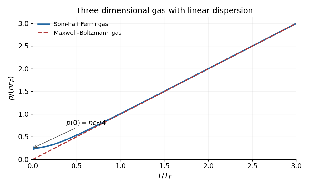
For spin-half fermions at $T=0$, all states up to the Fermi energy are occupied. With $g_s=2$,Integrating the occupied energy states givesThese are the corresponding ultrarelativistic ideal Fermi gas formulae with general slope $\alpha$. The nonzero ground-state internal energy and degeneracy pressure reflect the Pauli exclusion principle: particles cannot all occupy the lowest-momentum state. Formally extrapolating the classical equations gives $U,p\to 0$, but Maxwell–Boltzmann statistics is not valid at fixed positive $n$ as $T\to 0$.

At large $T$, the number equation gives $z\simeq N/Z_1\ll 1$, so expanding the Fermi-Dirac distribution recovers the Maxwell-Boltzmann distribution. A convenient crossover scale is the Fermi temperature,For $T\gg T_F$, both gases have $p\simeq n{k}_{B}T$. At fixed $n$, the Fermi curve begins at $p_0=n{ϵ}_F/4$, has zero initial slope, lies above the classical line, and approaches it at high temperature. For example its low-temperature expansion is $p/(n{ϵ}_F)=1/4+({\pi }^2/6)(T/T_F{)}^2+\cdots$. The plot evaluates the finite-temperature occupation integrals at fixed number density.

If the source's symbol $\mathbf{k}$ is interpreted literally as momentum rather than a wavevector, the state-space cell is $h^3/V$. In that convention replace $\alpha$ in the wavevector-based coefficients and energy scales above by $\hslash \alpha$. The dimensionless thermodynamics and the relation $p=U/(3V)$ are unchanged.

Chemotaxis supplies positive feedback: a local increase in bacterial density produces more attractant, whose gradient draws in more bacteria. Ordinary cell diffusion opposes aggregation. Chemical diffusion spreads the signal and removes very sharp gradients, while decay and logistic growth stabilize the uniform kinetics.

The dispersion relation from the preceding matrix makes the competition quantitative: the positive $D_n{D}_a{k}^4$ term stabilizes sufficiently short wavelengths, whereas the negative chemotactic contribution $-\alpha \chi k^2$ can destabilize intermediate wavelengths. Increasing cell diffusivity or chemical decay raises the attraction threshold. A growing allowed spatial mode produces correlated patterns in cell density and chemical concentration; the eigenvector relation $(\lambda +\beta +D_a{k}^2)\delta a=\alpha \delta n$ puts their peaks in phase for the growing real mode.

This predicts initial pattern formation. Nonlinear saturation and stability of the eventual pattern require the nonlinear equations, beyond the linear instability test.

Define $A=2\cot \alpha /3+8\mathrm{Re}/15$. The linearization about $h=1$ givesThe Galilean transformation $\xi =x-2t$, $\tau =t$ has ${\partial }_t={\partial }_{\tau }-2{\partial }_{\xi }$ and ${\partial }_x={\partial }_{\xi }$. It removes the leading advection, leavingFor a normal mode proportional to $e^{\sigma \tau +ik\xi }$, the second and fourth derivatives contribute $-k^2$ and $k^4$. The dispersion relation is thereforeFor $A>0$ and $S>0$, the unstable wavenumbers satisfy $0<|k|<\sqrt{A/S}$. In the laboratory coordinates, the temporal exponent is $\sigma -2ik$, so this linear stability calculation predicts growth together with downslope transport at dimensionless speed $2$.

Choose the rightgoing signed dispersion relation $\omega (k)=Nk/\sqrt{k^2+b_n^2}$. The horizontal phase velocity and group velocity areThe leftgoing branch has their negatives. For a convention using positive frequency at both signs of $k$, multiply each displayed speed by $\mathrm{sgn}k$. For every nonzero $k$, $0<c_g<c_p$ on the rightgoing branch; the horizontal group-speed bound for a confined internal wave is $c_g\le N/b_n$, approached as $k\to 0$.