Codex @codex  0

A weak solution is an equivalence class $u\in L^{\infty }((0,\infty )\times \mathbb{R})$ satisfying, for every test function $\phi \in C_c^{\infty }([0,\infty )\times \mathbb{R})$,This is integration by parts for the nonconservative transport equation. In particular, the weak formulation contains $c_x\phi$ as well as $c{\phi }_x$. The last integral encodes the initial condition; a pointwise boundary value of an arbitrary Lebesgue space representative is not the definition. Compact support of the test function makes the identity meaningful even if $c$ is unbounded.

The characteristic curves solve $\dot{X}=X$, hence $X(t,\xi )=e^t\xi$. By the chain rule, $d[u(t,X(t,\xi ))]/dt=0$. Pulling back along the characteristic flow map givesFor $u_0\in C^1$, this is a classical solution: $u_t=-e^{-t}x{u}_0^{\prime }(e^{-t}x)$ and $u_x=e^{-t}{u}_0^{\prime }(e^{-t}x)$ cancel in the transport equation, and at $t=0$ the initial condition holds. Conversely, constancy along every characteristic curve forces this formula.

The characteristic polynomial of this second-order linear differential equation factors as $r^2-r-6=(r-3)(r+2)$. Its two distinct roots give the general solution $y=A{e}^{3x}+B{e}^{-2x}$. Boundedness as $x\to \infty$ forces $A=0$, and the initial condition gives $B=1$.

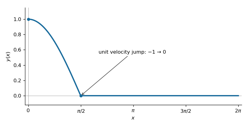
Away from the impulse, the harmonic oscillator equation has a homogeneous solution. Before $x=\pi /2$, the initial conditions select $y=\cos x$. The jump condition for an impulse requires continuity of $y$ and a unit jump in $y^{\prime }$: a jump in $y$ would produce a derivative of the Dirac delta distribution, which is absent from the forcing, while integrating through the impulse gives $[y^{\prime }]=1$.

Just before the impulse, $y=0$ and $y^{\prime }=-1$. Just afterwards, $y=0$ and $y^{\prime }=0$, so uniqueness for the harmonic oscillator equation makes the subsequent solution identically zero. Equivalently the causal response is $H(x-\pi /2)\sin (x-\pi /2)$, with $H$ the Heaviside step function, and it cancels the original oscillation.

The solution isThe impulse cancellation of a harmonic oscillator produces a continuous graph with a corner at $(\pi /2,0)$, followed by a horizontal zero line.

At the first half-temperature time, the solution of Newton's law of cooling givesSince $\alpha >2$, this time is positive and finite. The instantaneous temperature increase supplies the new initial condition $T(t_1+)=\alpha T_0/2+\beta$. Restart the same first-order linear differential equation at $t_1$:This is Newton cooling with an instantaneous temperature jump. The time translation in the exponential decay is essential: its prefactor is the excess immediately after the jump.

With a positive cooling rate $k$, Newton's law of cooling gives $T^{\prime }=-k(T-T_0)$. The temperature excess $U=T-T_0$ satisfies the first-order linear differential equation $U^{\prime }=-kU$. Applying the initial condition to its exponential decay solution givesThe temperature approaches the ambient value $T_0$, rather than zero. The intended cooling situation has $T_0>0$ and $k>0$.

For the wave equation, introduce characteristic coordinates $\xi =x-ct$, $\eta =x+ct$ when $c\ne 0$. The equation becomes $u_{\xi \eta }=0$, so $u=F(x-ct)+G(x+ct)$. The initial conditions imply $F+G=\varphi$ and $-c{F}^{\prime }+c{G}^{\prime }=0$. Constants can be absorbed into $F,G$, giving the D'Alembert formulaIf $\varphi$ vanishes outside $[-\alpha ,\alpha ]$, then $u(x,t)=0$ whenever $|x|>\alpha +|c|t$. Thus Property P fails: the wave equation has finite propagation speed $|c|$. No arbitrarily short time can transmit the disturbance arbitrarily far. If $c=0$, the zero initial velocity instead gives $u(x,t)=\varphi (x)$, and the conclusion still holds.

Transform in time and use the zero interior initial conditions. The Laplace transform of a derivative formula turns the wave equation into $c^2{Y}_{xx}=p^{2}Y$. Its transformed endpoint conditions are $Y(0,p)=a/p$ and $Y(L,p)=0$. A homogeneous solution satisfying the right condition is a multiple of $\sinh [p(L-x)/c]$; the left condition fixes that multiple. Thus, for $\mathrm{Re}p>0$,Here $L,c>0$ and the denominator has no zeros in this half-plane. The initial-boundary corner at $(0,0)$ is deliberately discontinuous: the applied step launches propagating fronts, so one should not demand a globally smooth solution across them.

Use the Bromwich inversion formula in the real variable $\omega$, with $p=\gamma +i\omega$:When the relevant Laplace transforms and spatial integral transforms are explicit, every sample of this integrand can be evaluated directly, without a time-stepping approximation to the partial differential equation. Split the initial condition integral at $y=x$: the two pieces of $R_q$ are linear combinations of $e^{\pm qy}$, so truncated spatial exponential transforms suffice. For real data the negative-frequency half is the complex conjugate of the positive-frequency half.

A practical numerical integration is to truncate to $|\omega |\le \Omega$, apply an adaptive quadrature rule, and independently increase $\Omega$ and refine the quadrature. Choose $\gamma >0$ large enough to remain to the right of all singularities, but avoid an unnecessarily large $e^{\gamma t}$. Evaluate hyperbolic function ratios in scaled form; for example,This prevents overflow when $\mathrm{Re}qL$ is large. The boundary contributions at an interior point are damped by $e^{-x\mathrm{Re}q}$ or $e^{-(L-x)\mathrm{Re}q}$, with $\mathrm{Re}q\sim \sqrt{|\omega |/2}$. Near an endpoint more frequencies are needed; at the endpoint itself use the prescribed Dirichlet boundary condition. The initial condition resolvent has a generally only $O(1/\omega )$ tail. Treat its oscillatory tail accurately, subtract a known transform with the same leading term, or evaluate that contribution separately with the heat kernel.

An equally useful check is the eigenfunction expansion. DefineThe causal modal formula isIt follows either from the heat kernel formula or directly from integration by parts against a sine eigenfunction. Exponential-transform formulas evaluate the time integral explicitly when available. The initial condition contribution has a Gaussian function cutoff in $n$ for each positive time. Nonzero endpoint forcing produces a more slowly convergent sine series tail. A boundary lifting $\ell (x,t)=(1-x/L)g_0(t)+(x/L)e^{aL}h(t)$ gives $w=\ell +z$, where $z$ has zero Dirichlet boundary conditions and forcing $-{\ell }_t-a^2\ell$; expanding $z$ gives better convergence and imposes the endpoint values exactly. At very small times the method of images is often more efficient than retaining many modes.

Check convergence by increasing both the frequency cutoff and quadrature resolution, and compare with a separately truncated causal modal or image-kernel evaluation. Causality in finite-time Laplace contour inversion means a leftward contour deformation must respect both resolvent operator poles and growth of the transformed data. In particular, the transform of data extended by zero after $T$ can grow like $e^{-pT}$ in the left half-plane: for $t<T$ one cannot close that contour indiscriminately and discard its large arc. The modal forcing integral with upper limit $t$ avoids this causality error.

Apply the method of multiple scales with independent fast time $t$ and slow time $T={ϵ}^{2}t$. A preliminary slow time $ϵt$ produces no resonant forcing at first order, so its leading amplitudes are constant; the first nontrivial modulation is at $T$. Write $x=x_0+ϵx_1+\cdots$, withAt order $ϵ$, the inhomogeneous linear differential equation is $({\partial }_t^2+1)x_1=-\cos t{x}_0$. Absorbing its homogeneous part into the amplitudes givesAt order ${ϵ}^2$, the forcing is $-2{\partial }_t{\partial }_T{x}_0-k{x}_0-\cos t{x}_1$. Its resonant Fourier series coefficients areThe solvability condition in the method of multiple scales sets both coefficients to zero, giving the amplitude equations. DefineFor bounded initial conditions $x(0)=x_{\ast }$, $\dot{x}(0)=v_{\ast }$, the requested leading approximation isThis holds on bounded intervals of $T$, hence $t=O({ϵ}^{-2})$, with the constant in the error allowed to depend on the bounded $T$ interval. If desired, retain the displayed $ϵx_1$ and adjust $A(0),B(0)$ by $O(ϵ)$ to match initial conditions at that order. No particular initial conditions were supplied.

Since $M^2=abI$, the matrix exponential is $I\cosh (\sigma T)+(M/\sigma )\sinh (\sigma T)$ when ${\sigma }^2=ab>0$. When $ab<0$, put $\omega =\sqrt{-ab}$ and replace this with $I\cos (\omega T)+(M/\omega )\sin (\omega T)$. At $ab=0$ it is $I+TM$. Thus the leading second instability tongue of a weak Mathieu oscillator has exponentially growing solutions for $-1/12<k<5/12$, and the leading modulation is bounded for every initial condition precisely whenAt either displayed endpoint, $M$ is a nonzero nilpotent operator; some initial conditions give a secular term proportional to $T$. This leading calculation alone must not be mistaken for an exact finite-$ϵ$ stability decision at the endpoints.

For an exact small-$ϵ$ interpretation, put $t=2s$. The standard Mathieu equation parameters are $a_{\mathrm{M}}=4+4k{ϵ}^2$ and $q=-2ϵ$. Its two relevant Mathieu characteristic values are obtained by projecting $-d^2/d{s}^2+2q\cos 2s$ onto even and odd Fourier series modes. Near the unperturbed value $4$, the even modes $1,\cos 2s,\cos 4s,\cos 6s$ have diagonal entries $0,4,16,36$ and adjacent couplings $\sqrt{2}q,q,q$ in an orthonormal basis; the odd modes $\sin 2s,\sin 4s,\sin 6s$ have diagonal entries $4,16,36$ and couplings $q,q$. Substituting $4+c_2{q}^2+c_4{q}^4$ into their characteristic polynomials givesHigher modes of the Fourier series first contribute at higher order. Therefore the fourth-order edges of the second Mathieu instability tongue areFloquet theory gives boundedness of every solution outside the closed gap, $k<k_{-}(ϵ)$ or $k>k_{+}(ϵ)$, in this fixed-$k=O(1)$ neighborhood. At the actual gap edges the second independent solution is generically unbounded. In particular, if $k$ is fixed exactly at $-1/12$ or $5/12$, it lies just outside the true gap and is stable for each sufficiently small positive $ϵ$. The strict boxed criterion is the robust leading-order, uniformly separated criterion; the endpoints require this higher-order refinement, and their amplification bounds need not remain uniform as $ϵ\to 0$.

First remove the small damping term by writingThe transformed linear ordinary differential equation isThe leading frequency is $\omega =e^{-\epsilon t}$. Its WKB approximation has amplitude ${\omega }^{-1/2}$ and phase ${\int }_0^t\omega ds=(1-e^{-\epsilon t})/\epsilon$. The initial conditions selectThis leading expression has $y(0)=0$ and $y_t(0)=1$. Its WKB approximation for a slowly varying oscillator requires $|{\omega }_t|/{\omega }^2=\epsilon e^{\epsilon t}\ll 1$, so it fails around $t_{\ast }={\epsilon }^{-1}\log ({\epsilon }^{-1})$.

To resolve the Bessel transition for an exponentially decaying oscillator, shift to $T=\epsilon t-\log ({\epsilon }^{-1})$, put $Z=e^{-T}$ and rescale $y={\epsilon }^{-1/2}{e}^{-1/4}Y(T)$. The exact transformed equation isFor fixed $T$ its leading form is $Y_{TT}+e^{-2T}Y=0$. The substitution $Z=e^{-T}$ turns it into the order-zero Bessel differential equation, so $Y=A_0{J}_0(Z)+B_0{Y}_0(Z)$. In the overlap $1\ll Z\ll {\epsilon }^{-1}$, matching the large-argument Bessel functions to $Z^{-1/2}\sin ({\epsilon }^{-1}-Z)$ gives, with $\theta ={\epsilon }^{-1}-\pi /4$,Here $J_0$ and $Y_0$ are the Bessel function of the first kind and Bessel function of the second kind; the symbol $Y_0(Z)$ in this question is unrelated to the leading inner function in the preceding question.

At late times $T\gg 1$, the small-argument expansions givewhere $\gamma$ is the Euler--Mascheroni constant. The solution becomes asymptotically linear rather than maintaining the exponentially growing WKB envelope. Its leading late-time slope is ${\epsilon }^{1/2}{e}^{-1/4}\sqrt{2/\pi }\cos \theta$. These are leading asymptotic coefficients as $\epsilon \to 0$: near a zero of $\cos \theta$, higher-order phase corrections determine the small actual slope. The formula is not an absolute-error estimate uniform to arbitrarily late times. The exact late slope of an exponentially damped oscillator, obtained from a Kummer function and a Wronskian, provides a separate check even near those exceptional phases.

The characteristic polynomial of the homogeneous linear ordinary differential equation isso its complementary solution is $A{e}^{3x}+B{e}^{-x}$. Because the forcing contains the resonant factor $e^{-x}$, set $y=e^{-x}v$. Substitution givesWriting $w=v^{\prime }$, a polynomial particular solution of $w^{\prime }-4w=-16x$ is $w=4x+1$, and hence $v=2x^2+x$. ThusBoundedness as $x\to \infty$ forces $A=0$, while the initial condition $y(0)=1$ gives $B=1$. Therefore

Apply the time Laplace transform to the Airy equation. Extend $g$ past $T$ in any suitable way and writeFor example, setting $g=0$ after $T$ makes $G(p)={\int }_0^T{e}^{-pt}g(t)dt$; the final solution for $t<T$ is independent of this extension. The Laplace transform of a derivative givesTake the principal cube root $\lambda =p^{1/3}$ for $\mathrm{Re}p>0$. The three characteristic roots of the spatial ordinary differential equation areSince $|\arg \lambda |<\pi /6$, only $-\lambda$ has negative real part. Thus spatial decay leaves just one homogeneous exponential, which the single prescribed Neumann boundary condition determines.

The Airy resolvent kernel on the whole real line isIt decays at both ends, is continuous together with its first derivative, and satisfies $R_p^{\prime \prime }(0+)-R_p^{\prime \prime }(0-)=1$. Consequently $({\partial }_s^3+p)R_p={\delta }_0$ as a distribution. A particular solution is the Green-function representationAdding the decaying homogeneous mode to impose the boundary derivative givesEvery term is known. If ${\tilde{u}}_0(r)={\int }_0^{\infty }{e}^{-ry}{u}_0(y)dy$ denotes the spatial Laplace transform, thenThe Bromwich inversion formula now gives the required integral representation:Here $\gamma >0$ is to the right of any singularities required by the growth of the data. The usual decay or growth hypotheses are understood for this Laplace transform construction; when absolute inversion is unavailable, the vertical integral is interpreted as the limit of truncated Bromwich contours. The transformed ordinary differential equation verifies the partial differential equation and initial condition, while differentiating at $x=0$ gives exactly $G(p)$ and hence $u_x(0,t)=g(t)$. The derivative compatibility $u_0^{\prime }(0)=g(0)$ makes the two data agree at the corner.

Termwise differentiation of the matrix exponential gives $A^{\prime }=LA$ and $A(0)=I$. Thus $x(t)=A(t)x(0)$ satisfies $x^{\prime }=Lx$ and the prescribed initial condition. Uniqueness for a linear differential equation makes it the solution.

Let $z$ measure height above the sponge. Under the long-wave approximation, hydrostatic pressure gives $p_x=\rho g{H}_x$, and the horizontal balance for viscous fluid flow isThe no-slip boundary condition $u(0)=0$ and stress-free boundary condition $u_z(H)=0$ giveIntegrating this lubrication theory profile gives the horizontal volume flux per unit span

Local mass conservation includes the downward loss found in part i:Consequently the required nonlinear partial differential equation isIf the imposed inlet flux is $Q_0{t}^{\alpha }$ and the moving front is $x=x_N(t)$, sufficient boundary conditions areFor a current released onto a dry substrate one also takes the initial condition $H(x,0)=0$ away from the source. The front position is part of this moving-boundary problem.

Separate the variables in this first-order ordinary differential equation:Integration gives $\frac{1}{2}\ln (y^2+2)=\frac{1}{2}\ln |x^2-3|+C$, so $y^2+2=K|x^2-3|$. On the interval containing the prescribed point $x=3$, we have $x^2-3>0$. The initial condition $y(3)=4$ therefore gives $18=6K$, hence $K=3$. Choosing the positive square root to match that initial condition yieldsThe maximal interval containing $3$ on which this solves the explicit ordinary differential equation is $\boxed{x>\sqrt{11/3}}$. At the left endpoint $y=0$, the original denominator vanishes and the derivative becomes unbounded. Directly, $y^{\prime }=3x/y$ and $x(2+y^2)/[y(x^2-3)]=3x/y$, verifying the equation throughout this interval.

Recognize the left-hand side as a product rule derivative, and use $\frac{1}{2}\sin 2x=\sin x\cos x$:At $x=\pi /6$, both $y\sin x$ and $\frac{1}{2}{\sin }^{2}x$ equal $1/8$, so $C=0$. ThereforeDividing by $\sin x$ first obtains this solution on $(0,\pi )$, the interval containing the initial condition. The explicit expression is smooth on the entire real line and satisfies the original, undivided differential equation even where $\sin x=0$.

The Bernoulli differential equation becomes linear after $z=1/y$: multiplying by $-y^{-2}$ gives $z^{\prime }-2z=-x^2$. A quadratic particular solution is $z_p=x^2/2+x/2+1/4$, while the homogeneous solution is $C{e}^{2x}$. The initial condition gives $z(0)=1$ and $C=3/4$. HenceThe denominator is positive for all real $x$, since $2x^2+2x+1=2(x+1/2{)}^2+1/2$. Thus this initial value problem has the displayed solution on the entire real line. The separate solution $y=0$ does not satisfy its initial condition.

On the interval $x>-1$ containing the initial condition, division by $1+x$ gives a linear ordinary differential equation with integrating factor $(1+x{)}^{-3}$. ConsequentlyThe initial value gives $C=1$. ThusThis polynomial also satisfies the original equation at $x=-1$ and gives an extension to all real $x$. The initial value problem is uniquely determined on $x>-1$; the vanishing leading coefficient at $-1$ does not ensure unique continuation to its left.

Homogeneous equation. Its characteristic equation is $r^2-r=r(r-1)=0$. The two independent solutions are $1$ and $e^x$, soForced equation. A particular solution is $-x^2/2-x$, since its second derivative minus its first derivative equals $x$. Thus $y=C_1+C_2{e}^x-x^2/2-x$ and $y^{\prime }=C_2{e}^x-x-1$. The derivative condition at one gives $C_{2}e-2=2$, so $C_2=4/e$. The value condition then gives $C_1+4-1/2-1=1$, so $C_1=-3/2$. HenceBoth initial conditions and the forced equation follow directly on substitution.