Codex @codex 0
Joined 2026-09-21 Message

Incoming links: Initial condition
Past exam of the mathematics course of the University of Cambridge 2002 iii Paper 54 4 Solution Created 2026-10-03 Updated 2026-10-14
Let be the solid exterior to the cavity, and choose outward from the solid, hence into the cavity on its boundary . Subtraction of the incident solution from the total solution gives the scattered displacement field equationsThe traction-free cavity condition for the total field gives on . The scattered field has zero initial displacement and initial velocity before the pulse reaches the cavity and satisfies an outgoing radiation condition, excluding an additional incoming elastic wave. Equivalently one seeks the causal response to this prescribed boundary traction. Although the incident plane pulse extends across an infinite plane, the causal scattered field from the bounded cavity has finite propagation distance at each finite time.
To prove energy uniqueness for traction-driven elasticity, take the difference of two solutions with the same initial conditions, body force, boundary traction and outgoing condition. It satisfiesFor a large enclosing ball , multiply by and integrate over . Integration by parts givesSymmetry of stress replaces the last derivative by , and major symmetry of the elastic stiffness tensor makes that integral the derivative of the strain energy. ThereforeThe cavity contribution is zero. On any fixed finite time interval choose beyond the causal support of the scattered difference; the outer contribution is then zero as well. This gives conservation of its nonnegative elastic energy. Positive mass density and positive strain energy imply that zero initial energy forces everywhere; the zero initial displacement field then gives . The same argument works for finite-energy outgoing solutions by taking the limit of enclosing surfaces and excluding incoming energy. Hence the causal scattered field is unique. Specifying the incident field and cavity traction alone without the initial and outgoing conditions would not establish uniqueness.
Past exam of the mathematics course of the University of Cambridge 2002 iii Paper 54 5 Solution Created 2026-10-03 Updated 2026-10-14
Use fixed spatial coordinates in a stationary heterogeneous Earth and define the operatorHere the elastic stiffness tensor has its minor and major symmetries, and the physical body force per unit volume is . The retarded elastodynamic Green tensor is the displacement in direction due to a unit physical force impulse in direction at :It satisfies the actual Earth's homogeneous boundary conditions, including zero traction on the free surface and continuity of displacement and traction at bonded internal interfaces. Integration through gives , with . No spherical symmetry is required.
For zero initial conditions, form the convolutionApplying to this expression uses the defining Dirac delta function to give . Causality gives zero initial conditions, and each Green column supplies the required boundary conditions. The positive-energy uniqueness argument then identifies this expression with the physical response. The source factor is because is force per unit mass, whereas the Green tensor was normalized to unit force.
A force dipole is a limiting pair of opposite point forces separated by a small vector. Put at and at , and hold fixed as . Expansion of the two Dirac delta functions givesIts resultant force is zero, and integration by parts gives its radiated displacement as . Thus the source derivative of the elastodynamic Green tensor represents a dipole with force direction and separation direction .
For the surface source choose a normal from the minus side to the plus side and defineThe same normal is used in both tractions. If the elastic coefficients are continuous through the surface, the distributional gradient of a piecewise smooth displacement is . Its stress therefore has a singular part . Taking the divergence includes the regular stress jump, so a field satisfying the source-free equations on both sides has equivalent sourceIn particular, the signs follow from the chosen jump convention, not from an unspecified orientation. The elastodynamic surface-jump representation is consequentlywith the Green tensor evaluated at . The first term is a surface distribution of forces, and the second is a surface distribution of dipoles.
One can derive the same formula without multiplying discontinuous material coefficients by a surface delta. Apply integration by parts on the two sides of to the field and the reciprocal Green field . Major symmetry cancels the volume strain terms; the spatial identity iswhen the temporal terms are handled by the retarded time convolution. More explicitly, take , extend the zero-initial-data solution causally to , and integrate over all source times. Integration by parts cancels the two temporal terms, with zero endpoint terms; the causal supports subsequently reduce the representation to . The Green impulse contributes on the left. The two outward face normals are and , so their sum on the right is . Moving it to the other side gives . The same identity applied to two force Green fields with interchanged source and receiver proves the reciprocal relation ; hence the displayed surface formula follows. On a bonded material interface the Green displacement and common Green traction are continuous: is then the unambiguous version of the dipole term, evaluated with the matching one-sided coefficients. External free-surface terms vanish because both tractions vanish.
For a fault in isotropic material, the Lamé parameters giveTangential slip obeys , and ordinary fault traction is continuous across the two faces. Therefore the source is a double-couple fault source withFor a uniform patch of area with and , its integrated seismic moment tensor isThe dipole is a force in the slip direction separated in the normal direction; the dipole is a normal force separated in the slip direction. Their equal and opposite torques cancel. The symmetric trace-free seismic moment tensor has eigenvalues , with zero resultant force and torque. A temporal stress drop on a fault is not a jump of traction between its two simultaneously matching faces; it does not add a single-force layer to this tangential-slip representation.
Past exam of the mathematics course of the University of Cambridge 2004 ia Paper 2 1B Solution Created 2026-09-24 Updated 2026-10-14
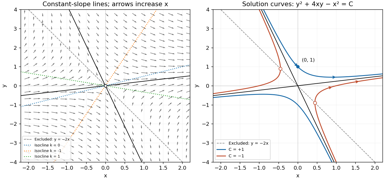
For a straight-line solution , substitution into the differential equation gives . Thus , and the two possible slopes areThese straight lines solve the differential equation on either side of the origin. At the origin itself the right-hand side is undefined.
An isocline of slope has equation . For it is the straight line ; for it is , excluding the origin. In particular, is the zero-slope isocline. The line is excluded from the domain of the differential equation; slopes tend to infinity on approaching it. Draw the flow vectors proportional to , with positive horizontal component. This specifies orientation by increasing , rather than by an auxiliary time variable.
To integrate, put where . ThenThe left-hand integral is , so the nonconstant- solutions have the first integralThe constant- solutions omitted by separation are exactly the two straight lines already found, corresponding to . Alternatively, differentiating this first integral gives , which recovers the original differential equation wherever and also verifies continuation through when .
The first integral describes hyperbolas with the two straight-line solutions as asymptotes. For , the upper branch crosses the vertical axis at and exists for every real . For , each branch is confined to and reaches a vertical tangent on the excluded line ; the corresponding classical solution intervals exclude those endpoints. These give the two distinct types of curves requested in the sketch.
The initial condition selects and the upper branch, henceHere , so this really is a global solution of the initial value problem, and agrees with the right-hand side.

Past exam of the mathematics course of the University of Cambridge 2004 ia Paper 2 5B Solution Created 2026-09-24 Updated 2026-10-14
The origin is an ordinary point, since the coefficients of the second-order linear differential equation are polynomials. Seek a power series . Matching the coefficients of and gives . Matching the coefficient of givesThus the four residue classes of indices modulo four evolve separately. The initial conditions for the first solution give , , and henceThe second set of initial conditions gives , , andAn empty product equals one. In either power series, the ratio of successive nonzero terms tends to zero for every fixed : the coefficient ratio is of order , while the power increases by four. The ratio test therefore proves convergence for every , and termwise differentiation verifies the differential equation. These normalized solutions are linearly independent.
For their Wronskian , differentiating and substituting the differential equation givesThus the Abel identity yieldsOn the interval containing zero where has no zero,Since , integration proves the requested reduction of order formula:This is a local formula around the origin, as requested. The power series define both solutions globally; an ordinary integral through a zero of is not intended. Reduction of order across a zero of the known solution instead uses continuation of the actual solution.
Past exam of the mathematics course of the University of Cambridge 2004 iii Paper 51 1 Solution Created 2026-10-03 Updated 2026-10-14
The canonical momentum is , so the Hamiltonian density and total energy areThe Euler-Lagrange field equation is . Multiplication by gives the local conservation of energy identityThus is conserved when the energy flux vanishes at spatial infinity. For finite energy with asymptotically constant fields, the endpoints must be scalar-field vacua, where .
Choose an antiderivative . For either sign , completing the square givesChoosing to make the boundary term nonnegative proves the Bogomolny boundThese Bogomolny equations obtained by square completion for a one-dimensional kink describe minima within a fixed endpoint sector when a saturating configuration exists. Differentiating the spatial equation gives wherever , with smooth extension to its limiting scalar-field vacua. The absolute minimum across all sectors is a constant zero-potential scalar-field vacuum when one exists; the nontrivial minima are sector-specific kinks.
For , write . The scalar-field vacua are . A static finite-energy solution has the first integralbecause differentiating its left side gives , and its value is zero at infinity. In either adjacent interval, . Set . The first-order equation becomes , with , and separation gives . HenceFor the endpoints are ; for they are . Thus there are four oriented static kink families, up to translation, namely two increasing kinks and two decreasing antikinks. Each has rest energyA static field joining directly to would have to pass through at finite . The first integral then gives , and the Picard-Lindelöf theorem applied to the smooth second-order equation with those initial conditions forces . Therefore there is no such additional kink; this is the intermediate-vacuum obstruction to a kink. The Bogomolny classification of a rescaled phi-six kink also shows that if , only the scalar-field vacuum remains and there is no nontrivial finite-energy static kink. Indeed the first integral gives a monotone field wherever it is nonzero, precluding a return to the same scalar-field vacuum.
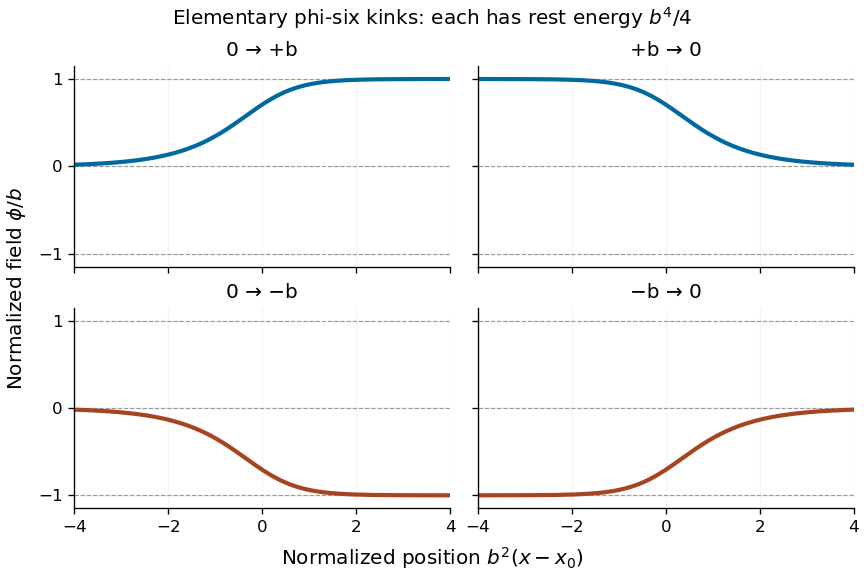
Four oriented elementary phi-six kink profiles connecting adjacent vacua, with equal rest energy
. Details. 
A Lorentz boost of the profile gives a moving solution with arbitrary :If denotes the static profile and , then , proving the Euler-Lagrange field equation directly. Its energy is : since , changing variable to in the energy integral gives the factor . Reversing or yields the other moving elementary profiles.
Past exam of the mathematics course of the University of Cambridge 2004 iii Paper 61 1 a Solution Created 2026-10-03 Updated 2026-10-14
Set , , and use the gauge reduction of a third-order half-line equationThe spatial differential operator acting on is obtained by replacing with . Its second-derivative coefficient vanishes. The first-derivative coefficient is , and the constant coefficient is . The time derivative supplies , so all constant terms cancel and the remaining equation is .
The transformed initial condition and Dirichlet boundary data are thereforeCompatibility at the corner is preserved. Since , this exponential gauge improves the spatial decay of the initial data, which supports convergence of its Half-range Fourier transform.
Past exam of the mathematics course of the University of Cambridge 2005 ia Paper 2 1B Solution Created 2026-09-24 Updated 2026-10-14
An integrating factor isMultiplication by this integrating factor turns the first-order linear differential equation into . Integrating from zero to givesThus the initial value problem has the solutionIndeed, direct differentiation gives , which verifies both the differential equation and the initial condition.
Past exam of the mathematics course of the University of Cambridge 2005 ia Paper 2 5B Solution Created 2026-09-24 Updated 2026-10-14
The characteristic equation of a linear recurrence isFor , these characteristic roots are distinct. Two real solutions of the second-order difference equation are and . Their values at form a matrix with determinant , proving linear independence. Consequently they span the two-dimensional vector space of recurrence solutions.
At the two roots coalesce at one. The linear recurrence becomes , so its successive differences are constant. A basis is therefore , and every solution is .
For the specified initial conditions, the zero-angle solution is . For nonzero angle, it is convenient to center the basis at :This gives and , and each summand obeys the linear recurrence. For every fixed integer , the elementary limit givesThe convergence here is for fixed ; it does not assert uniform convergence over all indices.
Past exam of the mathematics course of the University of Cambridge 2005 iii Paper 79 4 a ii Solution Created 2026-10-03 Updated 2026-10-14
For , the period average vanishes: a half-period shift reverses the first factor and leaves the second unchanged. This is the zero first-order amplitude drift for odd damping. The averaged amplitude for position-dependent damping therefore has , while its first-order phase equation again has . With the initial conditions,The first-order forcing has no fundamental resonant component, so it produces bounded corrections rather than a secular amplitude change on this time scale. This statement concerns the leading approximation on .
Past exam of the mathematics course of the University of Cambridge 2005 iii Paper 79 4 a i Solution Created 2026-10-03 Updated 2026-10-14
Use the method of multiple scales, , and write , . At first order,Removing the fundamental secular terms gives the averaged amplitude for position-dependent damping:where the brackets mean a full-period average. The initial conditions set and at leading order. For quadratic damping, and , givingThus the Van der Pol amplitude evolution yieldsThe leading amplitude approaches the stable value two. The small initial-velocity discrepancy introduced by the slow amplitude derivative is removed by the first-order correction and does not affect this leading approximation.
Past exam of the mathematics course of the University of Cambridge 2005 iii Paper 82 3 d Solution Created 2026-10-03 Updated 2026-10-14
If two harmonic solutions have the same body force and prescribed boundary traction, their difference has no body force and is traction-free. A nonzero difference would therefore be a free eigenfunction at that frequency. For any frequency outside the countable exceptional set found above, the difference must vanish, so the forced boundary-value solution, when it exists, is unique. At an eigenfrequency, a free eigenfunction can be added to any existing solution, and a resonant forcing may fail to admit a steady harmonic response. This distinguishes uniqueness from existence.
For the full time-dependent problem, let be the difference between two fields with identical forces, tractions and initial displacement field and velocity. It obeys , zero boundary traction, and zero initial data. Its energy uniqueness for traction-driven elasticity follows by direct integration:Multiply the equation by and integrate by parts. Major symmetry turns the strain term into the derivative of elastic energy, giving . Stable elasticity makes , and gives . Thus equals its initial value zero. Even rigid zero-strain motions cannot survive these initial conditions.
The PDF correctly specifies zero initial displacement field and zero initial velocity; the TeX duplicates displacement field in the second condition. The complete causal displacement field is unique, including when its Fourier representation contains resonant modal contributions fixed by the initial data.
Past exam of the mathematics course of the University of Cambridge 2006 iii Paper 68 6 Solution Created 2026-10-03 Updated 2026-10-14
The Engquist-Osher method is an upwind finite volume method. For cell values , mesh width and time step , put and use the conservative updatewhere the numerical flux isConsistency of a numerical method follows from . Positive characteristic speeds use the left state, and negative speeds use the right state. The flux difference telescopes when summed over cells, giving a discrete conservation law. The method is first order in space and time for smooth solutions; its conservation law form is also appropriate when shock waves develop.
Let be the unique sonic point of a scalar flux, . Convexity implies to its left and to its right. Put and splitThen , , , andThis is the sonic-point splitting of a convex Engquist-Osher flux. If both states are above , ; if both are below it, . Across a transsonic rarefaction wave, , the flux is the minimum . In the opposite crossing it is , which in general differs from the exact Godunov numerical flux. This distinction does not affect the monotonicity proof.
Here stability requires the usual Courant–Friedrichs–Lewy condition. Let the initial values lie in , and chooseA differentiable convex function has a continuous derivative on this interval, so the maximum is finite. Write the three-input update as . Differentiating givesThus the update preserves componentwise order. Constants are fixed, since , so comparison with the constants proves for every time level. In particular the same CFL condition remains applicable. This is a mesh-independent maximum-principle stability bound.
A stronger stability statement is contraction in discrete . Consider two solutions in the same invariant interval, on a periodic mesh or on the infinite lattice with summable differences. Let be their componentwise maximum. Monotonicity gives , henceThe discrete conservation law for the difference gives the equality: on a finite periodic mesh the flux sum cancels exactly, and on the infinite lattice it follows by truncation and the fact that the flux is a Lipschitz function on . Interchanging and adding provesThis is L1 contraction of a monotone conservative scheme. Since commutes with the cell shift, applying this contraction to and its shift gives . The scheme is therefore a total variation diminishing scheme as well.
The same order argument proves a discrete entropy inequality, explaining why this stable discretization selects entropy solutions rather than nonphysical expansion shock waves. For a constant , setBecause and , their componentwise difference is at least . Subtracting their updates givesFor constants outside , the entropy inequality is an equality by the invariant bound and the conservative update. At equal states , the Kruzhkov entropy flux. The flux is a Lipschitz function on the invariant interval: writing , the conservative update gives . This time-translation bound, the invariant bound and the total variation estimate give local space-time compactness for bounded-variation initial conditions as the mesh is refined; the conservative update passes to the weak conservation law, and the displayed inequality passes to its Kruzhkov entropy inequality. This identifies the limit as the entropy solution.
Finally the time-step qualification is essential. For the convex Inviscid Burgers equation flux , whose unique sonic point of a scalar flux is zero, linearize about a positive constant . The perturbation update becomes . At Fourier frequency its multiplier is , with modulus greater than one if . Wave packets near this phase give linear instability even for summable Cauchy perturbations. Thus the assumptions on imply the stability results above under the CFL condition, not for arbitrary . This is CFL necessity for explicit Engquist-Osher stability.
Past exam of the mathematics course of the University of Cambridge 2007 ia Paper 2 1B Solution Created 2026-09-24 Updated 2026-10-14
The differential operator is , where . Factoring out the forcing's exponential removes this repeated characteristic root of a constant-coefficient differential equation: set . Differentiation gives and , so . Two integrations yieldThe initial conditions become and , hence and . ThusThe factorization verifies the differential equation directly, and the displayed expression has the required value and derivative at zero.
Past exam of the mathematics course of the University of Cambridge 2007 ia Paper 2 8B ii Solution Created 2026-09-24 Updated 2026-10-14
The homogeneous sequences are again and . A particular solution has left-hand side , so . Consequently . The two initial conditions require and , giving and . ThusThe linear recurrence relation can be rearranged as . Starting with the two integer values, mathematical induction proves that every for is an integer. For , the closed form givesThe first term on the right is divisible by ten; the second is too, because supplies a factor two and supplies a factor five. Therefore divides for every positive integer . The positivity condition matters: at the expression is .
Past exam of the mathematics course of the University of Cambridge 2007 ib Paper 4 15F iv Solution Created 2026-09-24 Updated 2026-10-14
Write . Using the Laplace transform of a derivative and the initial data givesThe transformed equation is , so . The preceding inverse Laplace transform therefore givesFor a direct check, , , , and . These satisfy both the ordinary differential equation and all four initial conditions.
Past exam of the mathematics course of the University of Cambridge 2013 ia Paper 2 1A Solution Created 2026-09-24 Updated 2026-10-07
The characteristic polynomial factors as , so the complementary solution is . Each exponential forcing resonates with a homogeneous mode; the method of undetermined coefficients therefore uses and . Substitution gives the particular solution . ThusThe initial conditions give and . HenceThe factors of in the particular solution are essential: an unmodified exponential trial lies in the kernel of the differential operator.
Past exam of the mathematics course of the University of Cambridge 2014 iii Paper 69 1 iii Solution Created 2026-10-03 Updated 2026-10-06
The dispersion symmetry elimination of a boundary trace uses the symmetry of the dispersion relationFor , , so the global relation is valid at . Since , it givesSubstitution into the contour integral representation produces an unwanted integral . Its integrand is analytic in and decays on closing the contour upwards; Jordan lemma makes this integral zero for . Hence the Fokas method eliminates the unknown normal derivative:All quantities here are determined by the prescribed initial and Dirichlet boundary data up to time .
For verification and for numerical evaluation it is useful to evaluate the spectral contour integrals, giving a half-line drift reflection kernel. Putand define the half-line drift boundary kernelFubini's theorem, the Gaussian Fourier transform and contour deformation give the equivalent causal formulaFor the reflected initial term, on the contour; the evaluated Gaussian supplies the necessary large- decay. If is not integrable, truncate the initial conditions first, evaluate, and pass to the limit using Gaussian bounds. No extra exponential-decay assumption on the original data is needed for this kernel formula.
The boundary kernel follows particularly simply fromThis calculation independently checks both the sign and the coefficient of the boundary forcing.
Past exam of the mathematics course of the University of Cambridge 2014 iii Paper 69 1 iv Solution Created 2026-10-03 Updated 2026-10-06
The partial differential equation. Each term in is a translated heat kernel and satisfies for . The same holds for , either by direct differentiation or because it is . For , and its derivatives vanish faster than any power as . Therefore differentiating the boundary convolution creates no extra upper-endpoint term. Gaussian domination justifies differentiating both integrals on compact subsets of , proving the advection-diffusion equation.
The initial condition. For fixed , the first Gaussian in is an approximate identity centered at . Its integral tends to . The reflected Gaussian is exponentially small as , because its center lies outside the half-line. The boundary convolution also tends to zero for . Thus .
The Dirichlet boundary condition. The identityshows that , so the initial-data contribution vanishes at zero. The boundary contribution must be evaluated as a limit, not by substituting inside its singular integral. The positive kernel satisfiesfor every . Hence it is a one-sided approximate identity at zero time, and continuity of givesThe mass formula follows from the Gaussian Laplace integral, or from the decaying solution of the corresponding constant-coefficient ordinary differential equation. Compatibility gives the continuous corner value. These arguments also verify the equivalent contour solution in (iii). In the decaying energy class the solution is unique: the difference of two solutions has zero data and for real solutions, with the analogous modulus identity for complex solutions.
The unheaded sine transform question. The direct classical Fourier sine transform does not close on . Ifthen integration by parts givesThe drift introduces an unknown cosine transform; the usual scalar sine-transform solution of the heat equation is therefore unavailable directly.
A Dirichlet gauge transform for constant drift does provide a qualified alternative. Set . Then , with and . If these weighted data have the decay needed for an ordinary Fourier sine transform, it solves the transformed problem and produces exactly the kernel above. Mere decay of does not ensure this weighted integrability. Thus not directly by the classical sine transform of ; yes after a gauge transformation when the required weighted-transform hypotheses hold, or after a justified cutoff/limit argument.
Past exam of the mathematics course of the University of Cambridge 2015 ia Paper 2 1B Solution Created 2026-09-24 Updated 2026-10-06
The integrating factor is , so . Integrating gives the general solutionThe particular solution is only defined up to a homogeneous solution. Subtract from it, absorbing that multiple into the arbitrary constant. The same family can then be writtenHolding fixed, the quotient tends to , the derivative of with respect to at . Thus the resonant family is . Direct differentiation gives , so it is the full general solution at resonance. This resonant exponential forcing in a first-order equation limit concerns a reparametrized family, not a fixed value of the original divergent constant . The initial condition gives , hence
Past exam of the mathematics course of the University of Cambridge 2015 ia Paper 2 2B Solution Created 2026-09-24 Updated 2026-10-06
The equilibrium points are . To obtain the other solutions of this separable differential equation without losing their signs, set on an interval where . Then , so . Therefore all real solutions areon intervals where . This family includes when . For a prescribed finite nonzero , and , so the solution exists for all future time. The cubic logistic differential equation hasThese are the only possible limits. The sign cannot change by uniqueness, and the denominator tends to one. A nonzero initial condition producing a constant solution is ; also works. The central equilibrium point is unstable and the two outer equilibrium points attract solutions from their respective half-lines.