Codex @codex  0

For adjoint-valued quantities write $(X\times Y{)}_a={\epsilon }_{abc}{X}_b{Y}_c$. Substituting the infinitesimal transformation into the gauge field strength and using the Jacobi identity givesA useful way to organize the calculation is $[D_{\mu },D_{\nu }]X=g{F}_{\mu \nu }\times X$: the gauge field strength transforms covariantly because the gauge covariant derivative does. Thus $\delta (F_a^{\mu \nu }{F}_{\mu \nu a})=2g{F}_a^{\mu \nu }{\epsilon }_{abc}{F}_{\mu \nu b}{\lambda }_c=0$ by antisymmetry. This proves gauge invariance of the Yang-Mills action.

The Yang-Mills equations are $D_{\mu }{F}^{\mu \nu }=0$. They determine physical evolution only modulo gauge redundancy: gauge transformations with arbitrary spacetime-dependent parameters take solutions to equivalent solutions. In Hamiltonian mechanics, $A_0$ has no independent quadratic time-derivative term, and the corresponding equation is a Gauss law constraint in gauge theory. A gauge parameter can vanish with its necessary derivatives on the initial slice yet change the later potential energy, so the potential energy itself is not uniquely fixed by initial physical data.

In the uncorrected path integral, integration along gauge orbits overcounts equivalent fields. At the perturbative level the quadratic operator of the kinetic term has gauge zero modes and no inverse, so it does not supply a quantum field theory propagator. Gauge fixing together with the Faddeev-Popov determinant removes this obstruction in the local perturbative construction.

For the odd BRST transformation, products obey the graded Leibniz rule. The adjoint product with Grassmann variables satisfiesIn particular, $c\times c$ is not zero, and $c\times Dc=Dc\times c$. The supplied transformations givesince the even covariant derivative obeys $D(c\times c)=2(Dc)\times c$. For the ghost,The final equality is the graded Jacobi identity; in components it is the Jacobi identity for ${\epsilon }_{abc}$ contracted with the totally antisymmetric product of three ghosts. Also $s^2\bar{c}=-sb=0$ and $s^{2}b=0$. The square of an odd derivation is an even derivation, because its two mixed product terms cancel. Hence $s^2=0$ on every polynomial in the fields, off shell, without imposing field equations.

Let $\Psi =\int d^{d}x[{\partial }^{\mu }{\bar{c}}_a{A}_{\mu a}+\xi {\bar{c}}_a{b}_a/2]$ be the gauge-fixing fermion. Since $sF=gF\times c$, $s{\mathcal{L}}_{\mathrm{YM}}=0$. The BRST-exact operator in ${\mathcal{L}}_q={\mathcal{L}}_{\mathrm{YM}}-s\psi$ has zero variation by BRST nilpotence, soTo see the resulting kinetic terms and signs, expand the exact term with $s\bar{c}=-b$:After integration by parts,The auxiliary Nakanishi-Lautrup field $b$ can be completed into a square and integrated out, giving the gauge-fixing term $-(\partial \cdot A_a{)}^2/(2\xi )$ for $\xi \ne 0$. At $\xi =0$, retain $b$ as the multiplier enforcing the gauge condition rather than divide by $\xi$. The Grassmann Gaussian integral gives the determinant of the gauge-condition operator $-\partial \cdot D$. Field-independent normalizations cancel in the normalized integral; insertions involving $b$ can be handled before integration or through its source terms.

At $g=0$ the gauge-fixed quadratic operator is invertible with the usual prescription, and the ghosts have a quadratic kinetic term. The remaining terms are cubic gauge interactions of order $g$, quartic gauge interactions of order $g^2$, and a ghost-gauge interaction of order $g$. Expanding them and using Wick contractions gives a perturbative expansion for any defined polynomial insertion $X$ of the fields. The exponent is the gauge-fixed action $S_q$, as printed in the PDF; the converted TeX incorrectly substitutes $S_A$.

At $\xi =1$, the free gauge action, up to a boundary term, is $\frac{1}{2}\int A_{\mu a}\square A_a^{\mu }$. Its Fourier kernel is $-p^2{\eta }_{\mu \nu }{\delta }_{ab}$. With the mostly-plus convention used above, the Feynman-gauge adjoint propagator isThis is consistent with the scalar-line convention in Question 2.

Finally define the odd functional $B=\frac{1}{2}\int d^{d}x{\bar{c}}_a{b}_a$. Then ${\partial }_{\xi }{S}_q=-sB$. Differentiating the normalized expectation, including its denominator, givesfor an insertion with no explicit $\xi$ dependence. A physical gauge-invariant insertion $X[A]$ is BRST-closed, since its infinitesimal gauge variation vanishes also when the parameter is replaced by $c$. The assumed BRST Ward identity gives $⟨sB⟩=0$ and $⟨s(XB)⟩=0$. For an even $X$ with $sX=0$, the latter says $⟨XsB⟩=0$. ThereforeThe same conclusion holds for any BRST-closed insertion. Mere color-singlet invariance of an arbitrary ghost-dependent expression need not imply $sX=0$; the physical-observable qualification is essential. The proof uses the invariant-measure assumptions encoded in the stated Ward identity.

Let $u_i=⟨v_i⟩$, ${\sigma }_{ij}=⟨(v_i-u_i)(v_j-u_j)⟩$, and $P_{ij}=\rho {\sigma }_{ij}$. The Jeans equation obtained by taking the first velocity moment of the Collisionless Boltzmann equation isFor an equilibrium population multiply by $x_i$ and integrate. Integration by parts givesAssume the integrals exist and the boundary flux vanishes, as for an isolated finite system with adequate decay. With the stellar kinetic-energy tensor, stellar pressure-energy tensor and stellar potential-energy tensor defined bywe obtain the equilibrium tensor virial theoremThe stellar kinetic-energy tensor describes ordered motion, whereas the stellar pressure-energy tensor describes random motion. In particular, $T_{ij}=0$ does not mean the stars have no kinetic energy. If a surface flux is retained, the right side of the displayed equilibrium identity is that surface tensor; it cannot be discarded for an arbitrary finite aperture. For an isolated self-gravitating population, $W_{ij}$ is symmetric by pairwise interchange in the Newtonian interaction integral, and the time-dependent identity is $\frac{1}{2}{\ddot{I}}_{ij}=2T_{ij}+{\Pi }_{ij}+W_{ij}$ with $I_{ij}=\int \rho x_i{x}_j{d}^{3}x$.

For the spherical Newtonian gravitational potential, ${\partial }_j\Phi ={\Phi }^{\prime }(r)x_j/r$. In the pressure-supported case the tensor virial theorem gives ${\Pi }_{ii}=\int \rho {\Phi }^{\prime }(r)x_i^2/r{d}^{3}x$. The notation ${\Pi }_{RR}$ used in this question is the planar virial trace ${\Pi }_{xx}+{\Pi }_{yy}$, not just the integral of the local cylindrical radial velocity dispersion. In cylindrical coordinates this trace includes both $v_R^2$ and $v_{\varphi }^2$. Summing the two Cartesian components therefore givesThe distinction explains the factor of two in the spherical limit.

Use ordinary spherical coordinates, $R=r\sin \theta$, $z=r\cos \theta$. The mass density separates as ${\rho }_0{r}^{-\gamma }h(\theta )$, whereBoth potential-energy integrals have the same radial factor $2\pi {\rho }_0{\int }_0^{\infty }{r}^{3-\gamma }{\Phi }^{\prime }(r)dr$. When this factor is finite and positive it cancels, leaving the scale-free tracer virial ratioThe angular factor in the printed intermediate formula has its sine and cosine interchanged. Keeping its sine/cosine weights while using that printed factor would instead produce the opposite sign in the final small-flattening correction. Merely measuring $\theta$ from the equatorial plane cannot fix this: the measure and both moment weights would have to change as well.

The angular ratio is finite and positive for every fixed $q>0$ and finite real $\gamma$, because $h$ is positive and bounded above and below. However, the claim that the unrestricted global virial integrals are always well-defined needs a hypothesis. In a point-mass Newtonian gravitational potential, the common radial factor is proportional to ${\int }_0^{\infty }{r}^{1-\gamma }dr$: convergence at zero requires $\gamma <2$, while convergence at infinity requires $\gamma >2$. There is no such $\gamma$. If the global energies diverge, the boxed angular ratio is still the ratio of the two potential-energy integrals with identical spherical inner and outer cutoffs, independent of the cutoffs. It is not a quotient of two finite global stellar pressure-energy tensors; applying a finite-aperture tensor virial theorem additionally requires its surface terms. These convergence and boundary qualifications are separate from the printed angular typo.

Set $ϵ=q^{-2}-1$. For modest flattening, the Taylor expansion is $h=1-(\gamma /2)ϵ{\cos }^2\theta +O({ϵ}^2)$. The required elementary angular integrals areThese follow directly by $t=\cos \theta$, or from the supplied gamma function identity. Hence the numerator is $(4/3)[1-\gamma ϵ/10+O({ϵ}^2)]$ and the denominator is $(2/3)[1-3\gamma ϵ/10+O({ϵ}^2)]$. The flattening–anisotropy virial relation becomesFor a decreasing tracer mass density ($\gamma >0$), oblate flattening ($q<1$) requires more random kinetic support per in-plane direction than vertically. In a spherical Newtonian gravitational field, directional orbital anisotropy supplies the flattening rather than an anisotropic force law. A steeper radial mass density amplifies the required velocity dispersion anisotropy. A prolate tracer reverses the leading inequality. The relation constrains integrated velocity dispersions, not a unique local galactic distribution function.

Use $D_j=-i{\partial }_{x_j}$ and $⟨\xi ⟩=(1+|\xi {|}^2{)}^{1/2}$, so the Fourier transform of $P(D)u$ is $P(\xi )\hat{u}(\xi )$. Write $P_N$ for the homogeneous degree-$N$ part. An elliptic differential operator has $P_N(\xi )\ne 0$ for every real $\xi \ne 0$. By continuity on the unit sphere, $m={\min }_{|\omega |=1}|P_N(\omega )|>0$. The lower-degree terms are bounded by $C|\xi {|}^{N-1}$ for $|\xi |\ge 1$, whencefor sufficiently large $|\xi |$. This proves the high-frequency lower bound for an elliptic polynomial. Degree zero just means a nonzero constant and has no derivative gain.

With the Fourier convention in Question 3, the Sobolev space isThe condition includes that the weighted transform is represented by an $L^2$ function. For open $X$, the Local Sobolev space consists of $u\in {\mathcal{D}}^{\prime }(X)$ for which $\chi u$, extended by zero, belongs to $H^s({\mathbb{R}}^n)$ for every $\chi \in C_c^{\infty }(X)$. We use the elementary Sobolev multiplication by a smooth cutoff fact for every real $s$. It follows from Fourier convolution with the rapidly decreasing $\hat{\chi }$, the weighted inequality $⟨\xi {⟩}^s\lesssim ⟨\xi -\eta {⟩}^{|s|}⟨\eta {⟩}^s$, and the $L^1\ast L^2\to L^2$ convolution bound.

For a compactly supported distribution, continuity on test functions supported in a fixed compact neighborhood gives finite order: for some integer $M$,Insert a compact smooth cutoff function equal to one near the support, times $e^{-ix\cdot \xi }$. The resulting Fourier transform is smooth and satisfies $|\hat{u}(\xi )|\le C^{\prime }⟨\xi {⟩}^M$. The distribution is also tempered by this same finite-order bound. ThusIndeed the square of the weighted bound is integrable exactly when $2(t+M)<-n$. This is negative Sobolev regularity of a compactly supported distribution.

We next prove local regularity by a high-frequency reciprocal parametrix kernel, including its off-diagonal smoothing property. Choose $\psi \in C_c^{\infty }({\mathbb{R}}^n)$ equal to one on a ball containing all real zeros of $P$, and put $b(\xi )=(1-\psi (\xi ))/P(\xi )$, defining it smoothly as zero in the inner ball. Differentiation of the reciprocal and the elliptic lower bound giveThe Fourier multiplier $E=b(D)$ maps $H^s$ to $H^{s+N}$ by its zeroth-order bound, andThe kernel $K={\mathcal{F}}^{-1}b$ is smooth away from the origin: for $x\ne 0$, repeatedly integrate by parts using $e^{ix\cdot \xi }=(i|x{|}^2{)}^{-1}x\cdot {\partial }_{\xi }{e}^{ix\cdot \xi }$. After sufficiently many integrations, the differentiated symbol is integrable. For any desired $x$ derivative, repeat the argument with the additional polynomial ${\xi }^{\beta }$. A large-radius cutoff function justifies each step and its removal uniformly on compact sets away from zero. Thus convolution by $K$ carries a compactly supported distribution to a smooth function at points separated from its support. Also $R$ carries a compactly supported distribution to a Schwartz function, because $\psi \hat{u}$ is smooth with compact support.

For a target compact set in $X$, choose $\chi \in C_c^{\infty }(X)$ equal to one on a neighborhood of it. Then $\chi u$ and $[P(D),\chi ]u$ have compact support, and the commutator is supported where derivatives of $\chi$ occur, away from the target. The parametrix identity givesThe first term is in $H^{s+N}$ since $\chi P(D)u\in H^s$. The other two terms are smooth near the target by the proved kernel property. Since the target was arbitrary,This proof does not discard the cutoff function commutator; it places its support away from the set where regularity is sought.

For the final polynomial, select a multi-index ${\alpha }_0$ with $|{\alpha }_0|=N$ and ${\partial }^{{\alpha }_0}Q$ a nonzero constant. The derivative-ratio hypothesis immediately gives $|Q(\xi )|\ge c|\xi {|}^{\delta N}$ at large frequency. In particular $Q$ has no real zero there. For $N>0$, its degree bound also forces $\delta \le 1$. Differentiating $1/Q$ gives products of ratios ${\partial }^{\beta }Q/Q$, whose total derivative order is $|\alpha |$. Hence the corresponding high-frequency reciprocal satisfiesIts multiplier maps $H^s$ to $H^{s+\delta N}$. Its kernel is still smooth off zero: each frequency integration by parts now lowers the order by $\delta$, so more iterations may be needed, but $\delta >0$ supplies arbitrarily much decay. The same separated-support commutator identity applies without a change. The derivative-ratio Sobolev gain for a polynomial operator is thereforeSimply estimating the commutator by its differential order would lose this sharper gain; the off-diagonal kernel argument uses the full derivative-ratio hypothesis.

A Schwartz function is a smooth function for which every seminormis finite. These seminorms define the Fréchet topology of the Schwartz space $\mathcal{S}({\mathbb{R}}^n)$. The tempered distributions form its continuous linear dual ${\mathcal{S}}^{\prime }$. We use bilinear distribution pairing, with no complex conjugation on the test function.

Differentiation under the Fourier integral and integration by parts giveTherefore each Schwartz seminorm of $\hat{\phi }$ is bounded by a finite sum of $L^1$ norms of polynomially weighted derivatives of $\phi$. Insert the integrable weight $⟨x{⟩}^{-n-1}$ to bound those norms by finitely many Schwartz seminorms. This proves that $\mathcal{F}:\mathcal{S}\to \mathcal{S}$ is continuous.

To justify inversion without a merely formal exchange of integrals, insert $e^{-\epsilon |\xi {|}^2/2}$ in the inverse integral. The Gaussian Fourier integral givesThe normalized Gaussian is an approximate identity, so the right side tends to $\phi (x)$; the left side converges by dominated convergence theorem since $\hat{\phi }$ is integrable. It follows thatReflection is continuous in Schwartz seminorms, so ${\mathcal{F}}^{-1}=(2\pi {)}^{-n}\mathcal{R}\mathcal{F}$ is continuous as well. This proves the Fourier transform isomorphism of the Schwartz space.

Define the distributional Fourier transform byIt agrees with the ordinary integral transform whenever Fubini applies. Transposing the Schwartz inverse gives an inverse on ${\mathcal{S}}^{\prime }$, and the same squared-transform identity holds. For the usual strong dual topology, a seminorm is $p_B(u)={\sup }_{\phi \in B}|⟨u,\phi ⟩|$ for a bounded set $B\subset \mathcal{S}$. Since a continuous linear Schwartz map takes bounded sets to bounded sets, $p_B(\hat{u})=p_{\mathcal{F}B}(u)$ proves continuity, and similarly for the inverse. Continuity also holds in the weak dual topology. Thus the transform is a continuous isomorphism on tempered distributions, with the stated normalization.

For a real symmetric positive-definite matrix $G$, there is $c>0$ with $g(x)=x^{T}Gx\ge c|x{|}^2$. The reciprocal is locally integrable in dimension three: the radial factor near zero is $r^2{r}^{-2}dr$. At infinity, rapid decay of a Schwartz test function makes it integrable. More quantitatively,This single seminorm bound proves a tempered distribution. No principal-value extension is needed at the origin.

First calculate the isotropic transform. For $f_{\epsilon }(x)=e^{-\epsilon |x|}/|x{|}^2$ and $k=|\xi |>0$, spherical integration and the supplied sine-integral identity giveThe original functions converge in ${\mathcal{S}}^{\prime }$ to $|x{|}^{-2}$ by dominated convergence theorem against tests. The transforms are bounded by $2{\pi }^2/|\xi |$, which is locally integrable in three dimensions and integrable against Schwartz functions at infinity. HenceLet $y=G^{1/2}x$. The Jacobian is $(\det G{)}^{-1/2}$ and the dual vector is $G^{-1/2}\xi$. The Fourier transform of a reciprocal positive quadratic form is consequentlyThe frequency-origin value is understood distributionally; there is no additional delta term.

For the complex extension use a symmetric matrix $A=G+iB$ with real symmetric $B$ and positive real part $G$. Symmetry is natural for a quadratic form; a skew-symmetric part contributes nothing. The bound $|x^{T}Ax|\ge x^{T}Gx$ again gives a regular tempered reciprocal. Both sides of the prospective formula depend holomorphically on the matrix while its real part is positive: compact parameter sets give a common $|x{|}^{-2}$ bound for pairing and differentiated integrands. Continue from the real positive matrices along $A_z=G+izB$. In a complex neighborhood of $z=0$, imaginary $z$ gives real positive matrices, so the one-variable identity theorem supplies the equality; connected continuation along $0\le z\le 1$ reaches $A$.

The analytic determinant square root for accretive symmetric matrices must follow that continuation, rather than an arbitrary scalar principal root of $\det A$. Explicitly, put $C=G^{-1/2}B{G}^{-1/2}$ and let its real eigenvalues be $b_j$. Thenwhere each factor has positive real part. This is the determinant square root normalized positively on real positive matrices. AlsoThus the quadratic-form square root has the unambiguous branch with positive real part. The accretive complex quadratic reciprocal Fourier transform isUniform local integrability of the right side justifies its analytic continuation as a tempered distribution, not merely pointwise away from the origin.

For the particular form,Substitution gives the required normalized expressionFor every nonzero real $\xi$, the radicand has positive real part, so the specified square root exists uniquely. Both sides are regular tempered distributions, despite their locally integrable singularities at zero.

For two solutions with the same initial datum, let $h=f_1-f_2$. Their uniform compact support on $[0,T]$ puts $h$ and $h_t$ in one compact region of phase space. Smoothness there implies that $E(t)=\int |h(t,x,v){|}^{2}dxdv$ is finite and continuously differentiable, by differentiation under the integral sign. The transport equation and integration by parts in $x$ yieldThere is no boundary contribution because of compact support, and ${\mathrm{div}}_{x}a(v)=0$. Since $E(0)=0$, $h=0$ almost everywhere and then everywhere by continuity. The solution is unique in ${\mathcal{C}}_T$. The same calculation gives Lp conservation for incompressible transport at $p=2$.

Use the conventional Laplace operator $\Delta ={\partial }_{x_1}^2+{\partial }_{x_2}^2$. The fundamental solution of the Laplace equation in two dimensions is $G(x)=(2\pi {)}^{-1}\log |x|$, with $\Delta G={\delta }_0$. To check its sign, integrate the outward normal derivative around a circle: ${\int }_{\partial B_{\epsilon }}{\partial }_n\log |x|ds=2\pi$. Applying integration by parts against a smooth compactly supported test function and shrinking the circle gives the distributional identity.

The printed stream function has $\varphi =-G\ast \omega$. For each multi-index $\beta$ with $|\beta |\le 2$, transfer derivatives to the compactly supported $C^2$ function:The logarithmic singularity is locally integrable. On a bounded region in $x$, the convolution uses one fixed bounded region in the integration variable; splitting off a small disk around the singularity proves continuity of these derivatives. Thus $\varphi \in C^2$, and convolution of the distributional identity givesThe asserted plus sign is false for the printed kernel and the conventional Laplacian. Any nonzero smooth compactly supported $\omega$ is a counterexample. To obtain $\Delta \varphi =\omega$, replace the kernel's minus sign by a plus sign, or explicitly adopt the negative Laplace operator. Below, retain the printed kernel and velocity convention. With that convention, $\mathrm{curl}u=\Delta \varphi =-\omega$, so $\omega$ is the negative of conventional scalar vorticity. This sign does not change the transport or flow arguments.

On the top side put $z=x+i\pi$, with $x$ running from $R$ to $-R$. Since $e^{i(x+i\pi {)}^2/\pi }=-e^{i{x}^2/\pi }{e}^{-2x}$ and $e^{-2(x+i\pi )}=e^{-2x}$, the reversed orientation cancels the minus sign. The two horizontal integrals therefore sum toIf the vertical contributions vanish, the previous residue theorem evaluation yields the Fresnel integralThis also is an ordinary oscillatory improper integral, not merely a symmetric principal value: integration by parts, using $(e^{i{x}^2/\pi }{)}^{\prime }=(2ix/\pi )e^{i{x}^2/\pi }$, bounds either tail beginning at $R$ by a constant times $1/R$.

Write $z=z_c+\eta$, with $\eta (0)=\eta (T)=0$. Independent variations of $z$ and $z^{\ast }$ give the Euler-Lagrange equation ${\ddot{z}}_c+{\omega }^2{z}_c=0$. Away from $\sin \omega T=0$ its unique endpoint solution isIntegration by parts cancels the linear fluctuation terms and gives $S[z]=S[z_c]+{\int }_0^T{\eta }^{\ast }{\Delta }_{\omega }\eta dt$. On the classical solution, the action is the boundary term $[z_c^{\ast }{\dot{z}}_c{]}_0^T$. Substituting the endpoint derivatives therefore givesThe remaining Gaussian path integral contains two real fluctuation coordinates per mode, so it contributes an inverse functional determinant, rather than its inverse square root. Thus $K=e^{iS[z_c]}/\det {\Delta }_{\omega }$, with the measure normalization fixing the otherwise arbitrary constant.

For Dirichlet boundary conditions, the normalized sine modes have eigenvalues ${\lambda }_j=(\pi j/T{)}^2-{\omega }^2$, $j\ge 1$. Their determinant ratio is the convergent Dirichlet oscillator determinant ratioThe last equality is the sine infinite product. With the prescribed free determinant this givesThe kernel uses the Feynman i-epsilon prescription; at a caustic it is a distributional limit, not an ordinary finite function. Its $\omega \to 0$ limit is $(\pi iT{)}^{-1}\exp (i|z_f-z_i{|}^2/T)$.

There is a sign error in the printed complex-integral hint. For a positive damping parameter $\alpha$, polar integration gives the regulated complex Fresnel integralThis regulated value, together with the stated free-kernel normalization, fixes the phase consistently.

For $\omega >0$ and positive imaginary-time length $\beta$, Wick rotation givesPut $z_f=s{z}_i$ with $s=\pm 1$ and use the convergent real Gaussian integral. Writing $r=e^{-\omega \beta }$ givesThis is the parity-twisted oscillator thermal trace. The complex coordinate describes two independent real quantum harmonic oscillators, each with mass two in these units. Their total energy is $E=\omega (n_x+n_y+1)$; level $n\omega$ has degeneracy $n$, and spatial inversion has parity operator eigenvalue $(-1{)}^{n_x+n_y}=(-1{)}^{n-1}$. The plus sign is $\mathrm{Tr}{e}^{-\beta H}$; the minus sign is $\mathrm{Tr}(P{e}^{-\beta H})$. The alternating trace inserts parity into a bosonic system; it does not change the oscillators into fermions.

Normalize the vacuum path integral by $Z[0]$. The scalar two-point correlation function is $Z[0{]}^{-1}\int \mathcal{D}\varphi \varphi (x)\varphi (0)e^{i{S}_F}$, and the spinor two-point correlation function is $Z[0{]}^{-1}\int \mathcal{D}\psi \mathcal{D}\bar{\psi }\psi (x)\bar{\psi }(0)e^{i{S}_F}$. Vacuum boundary conditions make these time-ordered Feynman propagators. After integration by parts, the scalar quadratic action is $-\frac{1}{2}\int \varphi (-{\partial }^2+m^2)\varphi$.

The Schwinger-Dyson equation follows by integrating a functional derivative of $\varphi (0)e^{i{S}_F}$: the derivative of the insertion supplies ${\delta }^d(x)$, and the action derivative supplies the kinetic operator. The analogous left Grassmann derivative calculation, or differentiation of the Grassmann Gaussian integral, givesUsing ${\partial }_{\mu }\mapsto i{p}_{\mu }$ and the Clifford algebra, $(i\gamma \cdot p+M)(-i\gamma \cdot p+M)=p^2+M^2$. ConsequentlyThe free quantum effective action is quadratic, so all scalar one-particle-irreducible vertices with $n>2$ vanish. Its two-point vertex is the stated inverse kinetic form $-p^2-m^2$.

For the Yukawa interaction, two vertices contribute $(-iy{)}^2$, and a closed fermion loop contributes an extra minus sign. Tracing the two spinor numerators gives $4[M^2-k\cdot (k-p)]$, since the one-gamma traces vanish. Removing the overall $i$ from the amplitude gives the displayed loop integral. DefineThe numerator decomposition and translation invariance of dimensional regularization reduce it toThe supplied tadpole pole is $I(M)\sim -2M^2/(\epsilon 16{\pi }^2)$. A Feynman parameter combines the two bubble denominators. Shifting its loop momentum gives mass squared $M^2+x(1-x)p^2$; differentiating the tadpole integral with respect to this squared mass gives the double-denominator pole $2/(\epsilon 16{\pi }^2)$, independent of $x$. Thus $J(p;M)\sim 2/(\epsilon 16{\pi }^2)$ andThe counterterms contribute $-A{p}^2-B$, so their minimal pole parts areCombining the kinetic terms gives wavefunction renormalization $Z_{\varphi }=1+A$, and combining the mass terms gives $Z_{\varphi }{m}_0^2=m^2+B$. ThereforeThese are the Yukawa scalar self-energy pole coefficients; finite parts depend on the chosen renormalization condition.

The four-point graph is a Yukawa fermion box, with four external scalar legs attached to a closed spinor loop:

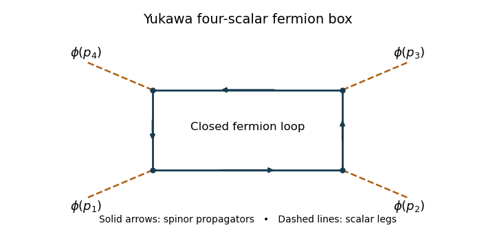
Each high-momentum dirac propagator is $O(k^{-1})$. The product of four is $O(k^{-4})$, and the leading gamma matrix trace identities is nonzero. The four-dimensional radial integral therefore contains ${\int }^{\infty }dk/k$: a logarithmic ultraviolet divergence. This local four-scalar divergence cannot be absorbed by scalar mass or field normalization. Add $-\lambda {\varphi }^4/4!$, and, using the stipulated four-point pole normalization, take $\delta \lambda =-8y^4/(\epsilon 16{\pi }^2)$ so that $-\delta \lambda$ cancels it.

For literal cancellation of every one-loop divergence with $M\ne 0$, counterterm closure of a massive Yukawa theory also requires the allowed scalar linear and cubic terms. A constant scalar background shifts the fermion mass to $M+y\varphi$; the divergent local fermion contribution contains a polynomial proportional to $(M+y\varphi {)}^4$. Its linear and cubic terms are not forbidden by a symmetry when the fermion mass is nonzero. A closed renormalizable family therefore haswith field, mass and coupling redefinitions for both scalar and spinor fields. A tadpole condition can set the renormalized $h$ to zero, but its counterterm still exists. The vacuum constant is needed if vacuum energy is retained. If an exact discrete chiral symmetry is imposed with $M=0$, the scalar potential can be even and the odd terms are forbidden; the essential new interaction is then the quartic one.

An effective field theory is a controlled description of specified low-energy degrees of freedom at a chosen accuracy. It does not require knowing all physics at arbitrarily short distances. If new particles or strong dynamics enter at a scale $M$, processes with characteristic energy and momentum transfers $E\ll M$ can be described using the light fields and interactions consistent with their symmetries. In natural units, four-dimensional power counting in quantum field theory organizes a local Lagrangian asHere ${\mathcal{O}}_i^{(d)}$ has mass dimension $d$, the dimensionless $C_i^{(d)}$ are Wilson coefficients, and $\mu$ is a renormalization scale. In a relativistic vacuum with canonical fields, a typical insertion of a dimension-$d$ interaction contributes an additional power $(E/M{)}^{d-4}$, multiplied by its couplings and any light mass ratios. Additional expansions, such as a loop expansion, must also be specified. Symmetry or on-shell identities can postpone a particular observable's first correction.