Codex @codex  0

Let $y$ be a smooth constrained minimizer. For any smooth variation $h$ vanishing at the endpoints, use the normalized admissible curve $y_{\epsilon }=(y+\epsilon h)/\sqrt{J[y+\epsilon h]}$. Since $J[y]=1$, differentiating at zero givesIn particular this holds for every compactly supported test function $h$ in $(0,1)$. Integration by parts and the fundamental lemma of the calculus of variations givewhich is the required Bessel differential equation with $\boxed{\lambda =I[y]}$. The lemma used here says that a continuous function whose integral against every compactly supported smooth test function is zero must itself vanish. No multiplier-existence theorem is needed: the explicit normalization produces the variation directly.

The endpoint $0$ causes no divergent energy for these variations: smoothness and $y(0)=h(0)=0$ imply $y,h=O(x)$. Also $J[v]>0$ for every nonzero admissible $v$, and $v/\sqrt{J[v]}$ has unit $J$ and energy $I[v]/J[v]$. Thus minimizing $I$ with $J=1$ is equivalent to minimizing the scale-invariant Rayleigh quotient $I/J$. The zero function is excluded whenever this quotient is written.

An energy measurement selects the ground state with probability equal to the squared inner product with ${\psi }_1$. Using $N=\sqrt{3}/L^{3/2}$ and integration by parts,ThusThe full Fourier sine series has $c_n=(-1{)}^{n+1}\sqrt{6}/(n\pi )$, so ${\sum }_n|c_n{|}^2=(6/{\pi }^2){\sum }_n{n}^{-2}=1$, an independent wavefunction normalization check. However $E_n|c_n{|}^2=3{\hslash }^2/(m{L}^2)$ for every $n$, hence ${\sum }_n{E}_n|c_n{|}^2$ diverges. This explicitly verifies the infinite-energy expectation qualification in part (b), without invalidating the individual projection probabilities.

Vary $S=\int L(q,\dot{q},t)dt$ with fixed endpoints. Integration by parts gives $\delta S=\int {\sum }_i[L_{q_i}-d{L}_{{\dot{q}}_i}/dt]\delta q_{i}dt$, hence the Euler-Lagrange equations. Define $p_i=L_{{\dot{q}}_i}$ and, assuming an invertible velocity-momentum relation, $H=p\cdot \dot{q}-L$. The equivalent action is $\int (p\cdot \dot{q}-H)dt$. Independent variations of $p$ and $q$ yieldBoundary terms vanish for fixed endpoint coordinates; constraining momenta independently at the same endpoints is unnecessary. Singular Lagrangians require constraint analysis instead of this unconstrained Legendre transform.

Split the sine into exponentials. The $e^{iz}$ term closes in the upper half-plane and picks up the pole $ia$, giving $2\pi i{e}^{-a}$; the $e^{-iz}$ term closes clockwise below and encloses no pole. Jordan's lemma applies to these separate contours. HenceTo pass to $a\downarrow 0$ without an invalid dominated-convergence argument on an infinite interval, pair positive and negative $x$ first: the imaginary part is odd and the real part is $2{\int }_0^{\infty }x\sin x/(x^2+a^2)dx$. On a bounded interval the limit is harmless, while integration by parts bounds the oscillatory tail uniformly for $0<a\le 1$. This gives the convergent improper Dirichlet integral $\boxed{{\int }_{-\infty }^{\infty }\sin x/xdx=\pi }$.

Multiply hydrostatic equilibrium by $4\pi r^{3}dr$ and integrate from centre to surface. Integration by parts, neglecting external surface pressure, givesFor an ideal gas with a constant adiabatic index, $U=\int PdV/(\gamma -1)$. ConsequentlyA fully ionized, nonrelativistic monatomic gas has $\gamma =5/3$, provided gas rather than radiation or degeneracy dominates the thermal equation of state. It then obeys $\boxed{2U+\Omega =0}$ and $E=U+\Omega =-U=\Omega /2$.

Added nuclear heat initially raises pressure and causes expansion. The expansion makes gravitational energy less negative and can lower the temperature of the self-gravitating gas, reducing the temperature-sensitive fusion rate. Conversely, a small contraction can raise the core temperature and increase burning. This negative feedback explains stable main-sequence burning in an ordinary nondegenerate stellar core; a degenerate core need not respond the same way.

Before hydrogen ignition, a cloud loses energy by radiation and contracts. Its gravitational energy decreases; for the ideal-gas virial relation, roughly half the released binding energy heats the gas and half is radiated. Heating continues until nuclear reactions can balance the luminosity, explaining the Kelvin-Helmholtz phase of pre-main-sequence evolution.

The effective adiabatic response varies with ionization, molecular dissociation, radiation pressure and degeneracy. Partial ionization can absorb compression energy and lower the local first adiabatic exponent below $4/3$, encouraging compressibility, convection and pulsational instability. A local outer layer with $\gamma \le 4/3$ does not by itself prove global collapse: ordinary stars have ionization layers of that kind. The dynamical stability criterion concerns a suitable pressure-weighted global response and its coupling to the eigenmode; an extended star with an effectively global exponent below $4/3$ can be dynamically unstable.

Let the boundary split into a displacement part ${\Gamma }_D$ and a traction part ${\Gamma }_N$. The linearized stored elastic energy functional isIts corresponding total potential subtracts the work of fixed body and surface loads:The problem in the calculus of variations is to minimize $\Pi$ among admissible displacements with $u=u_D$ on ${\Gamma }_D$. For a stable quadratic elastic energy this is the usual energy minimization formulation. Its stationarity condition suffices to derive equilibrium.

Vary by $u+sv$, with $v=0$ on ${\Gamma }_D$. Major symmetry combines the two differentiated quadratic terms, givingIntegration by parts, first with test functions compactly supported in the interior, gives $-\mathrm{Div}{S}^{\mathrm{lin}}=f$. Then arbitrary traces on ${\Gamma }_N$ give the natural traction condition. The complete boundary value problem isFor a homogeneous hyperelastic material the elasticity tensor is constant. In isotropic linear elasticity the constitutive equation is $S^{\mathrm{lin}}=\lambda \mathrm{div}uI+\mu (Du+D{u}^T)$, giving the familiar Navier-Cauchy equation $-\mu \Delta u-(\lambda +\mu )\nabla \mathrm{div}u=f$.

The given probability density function is that of a beta distribution with parameters $r$ and $n-r+1$. We can derive the required moments directly rather than assuming the beta moment formulas. For an integer $j\ge 0$, the Euler beta function givesHere $B(a,b)=(a-1)!(b-1)!/(a+b-1)!$ for positive integers $a,b$; this identity also follows by repeated integration by parts. Taking $j=1,2$ yieldsSubtract the square of the first moment from the second to obtain the variance:These are exact finite-sample identities for each uniform order statistic.

Use the corrected piecewise-deterministic Markov process from part (b). For a smooth test function $f$, its time-dependent infinitesimal generator isIndeed, over an interval of length $h$, deterministic motion contributes $ha(t,x)f^{\prime }(x)$, while a jump has probability $h\alpha (x)+o(h)$ and changes the conditional mean of $f$ by $K_{t}f(x)-f(x)$. Terms involving both drift and a jump contribute only to the remainder. Thus $P_{t,t+h}f=f+h{L}_{t}f+o(h)$.

The Dynkin formula, or this infinitesimal expansion integrated against the current probability distribution, gives the weak evolution identityTake $f\in C_c^{\infty }(\mathbb{R})$, so integration by parts has no boundary contribution. Assuming the displayed jump integrals are finite, Fubini's theorem givesConsequently the forward equation of a piecewise-deterministic Markov process isHere $A_t=L_t^{\ast }$ is the formal adjoint operator acting on probability density functions. Its terms are transport, loss from $x$, and incoming mass from every $y$. In particular, the incoming rate is $\alpha (y)$, evaluated at the departure state. The operator denoted $A$ in the source is generally time-dependent. Because $\int m_t(y,x)dx=1$, the gain and loss integrals cancel; with vanishing transport flux at infinity, $\frac{d}{dt}\int p_t=0$.

The deterministic initial state in part (b) does not actually yield an everywhere smooth full density. For finite times the no-jump contribution is the positive measurewhere ${\delta }_z$ is the Dirac measure at $z$. Smooth jump destination probability density functions cannot remove this positive atom. The density equation above is therefore conditional on the extra density hypothesis, for example with a suitable random initial probability density function. For the specified fixed initial state, write ${\nu }_t$ for the whole probability measure and use insteadThis weak measure evolution includes both the atom and any continuous component. It becomes the displayed partial differential equation whenever ${\nu }_t(dx)=p_t(x)dx$ with the assumed regularity. It does not describe the literal hidden-reset construction without the correction in part (b).

Take $f$ in the generator domain $D(L)$. The semigroup commutation with its unbounded generator implies $P_{t}f\in D(L)$ andIndeed, applying the bounded operator $P_t$ to the difference quotient at zero gives the right derivative $P_{t}Lf$; strong continuity gives the full orbit derivative for $t>0$. Now integration by parts in the Bochner integral yieldsThe boundary term at infinity vanishes because $\Vert e^{-\lambda t}{P}_{t}f\Vert \le e^{-\lambda t}\Vert f\Vert$. The derivative integral exists as a Bochner integral, since its integrand is bounded in norm by $e^{-\lambda t}\Vert Lf\Vert$.

Multiplying this identity by $\lambda$ givesPart (b) applies to the fixed vector $Lf\in E$, soThe bounded operators $L_{\lambda }={\lambda }^2{R}_{\lambda }-\lambda I$ are the Yosida approximation of the semigroup generator. The proof only applies the unbounded operator $L$ to $f\in D(L)$; the contraction and limit arguments then act on the ordinary vector $Lf$.

For $\lambda >1$, use $x/\lambda \ge 1$ on the tail:This proves the requested Gaussian tail bound.

The subsequent printed maximum inequality is false as stated. For $n=1$ its integrand never reaches one, and its right-hand side isBut for two independent absolute standard normal variables, using their common distribution function $F(x)=2\Phi (x)-1$ and the standard normal density $\phi$,The middle step is integration by parts with ${\phi }^{\prime }=-x\phi$. Thus no proof of the displayed source inequality can hold for all its stated indices.

The correct tail integral formula for expectation isA valid union bound givesIn particular, for $x>1$ this is at most $\min (1,C_n{e}^{-x^2/2})$, where $C_n=2^{n+1}/\sqrt{2\pi }$. This corrected estimate proves the intended summability in part (c), without silently replacing the source formula.

Along $x=Vt+x_0$, the phase is $t\Phi (k)+k{x}_0$, with $\Phi (k)=kV-\omega (k)$. Graphically, a line of slope $V$ intersects the dispersion curve transversely except where it is tangent. On a transverse region, neighboring wavenumbers acquire order-one phase differences over a width $\Delta k\sim t^{-1}$, so cancellation leaves an $O(t^{-1})$ contribution. More formally, integration by parts usesand gives that order when the amplitude and its derivative are integrable and ${\Phi }^{\prime }$ is bounded away from zero on the region.

At a nondegenerate tangent point $k_{\ast }$, ${\Phi }^{\prime }(k_{\ast })=0$, equivalently $\boxed{V={\omega }^{\prime }(k_{\ast })}$, and $\Phi (k)=\Phi (k_{\ast })-{\omega }^{\prime \prime }(k_{\ast })(k-k_{\ast }{)}^2/2+\cdots$. Coherent wavenumbers now occupy width $O(t^{-1/2})$, yielding the stationary-phase contributionThese are the packets whose group velocity follows the observer. The displayed decay rates require the usual regularity and nondegeneracy hypotheses; $A\to 0$ alone is not a complete analytic hypothesis, and a vanishing amplitude or degenerate stationary point changes the leading order.

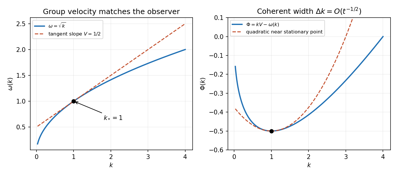
For deep water take a velocity potential satisfying Laplace's equation below the undisturbed surface and decaying with depth. A Fourier mode has vertical factor $e^{|k|z}$. The linearized kinematic and dynamic surface conditions are ${\eta }_t={\varphi }_z$ and ${\varphi }_t+g\eta =0$ at $z=0$. ThusRelease from rest gives ${\overline{\eta }}_t(k,0)=0$, so inversion of the Fourier transform givesEvenness of the initial profile makes its transform even and the reconstructed surface even; the same formula also works without that symmetry when the usual reality condition holds.

Split the cosine into its two time phases. Along the moving observer, their stationary conditions are $\pm {\omega }^{\prime }(k)=V$, where $\omega (k)=\sqrt{g|k|}$. Since $|{\omega }^{\prime }(k)|=\sqrt{g}/(2\sqrt{|k|})$, for $V\ne 0$,These are the possible dominant stationary-phase packets, provided the initial Fourier amplitude at the selected wavenumber is nonzero. For $V=0$ there is no finite nonzero stationary wavenumber; the formula must not be applied by division by zero.

Split $I$ into the two tails and the interval $|k-k_{\ast }|<\delta$. On each tail ${\psi }^{\prime }$ has a fixed nonzero sign, so changing variable to $s=\psi (k)$ produces a nonstationary Fourier integral. Under the usual decay and regularity needed for integration by parts, these pieces are $O(t^{-1})$.

Near the nondegenerate stationary point, make the signed local changeIt has $dk/dz=1$ at zero and makes the phase exactly $\psi (k_{\ast })+{\psi }^{\prime \prime }(k_{\ast })z^2/2$. The transformed amplitude tends to $f(k_{\ast })$. Scale $z$ by $t^{-1/2}$ and use the Fresnel integral to obtainThe $O(t^{-1})$ tails are smaller than this leading stationary contribution. If ${\psi }^{\prime \prime }(k_{\ast })<0$, complex conjugation of the Gaussian phase changes the phase correction to $-\pi /4$ and replaces the second derivative by its absolute value:When the leading coefficient is nonzero this may be written as an asymptotic equivalence. For full rigor, continuity of an arbitrary amplitude alone is not sufficient for the stated nonstationary $O(t^{-1})$ rate, nor does it ensure convergence of an infinite integral. Piecewise differentiability with integrable derivative, bounded variation, or an equivalent localization/decay hypothesis supplies the usual missing assumption. The exponentially decaying beam amplitude below has the required piecewise regularity.

Take the nondegenerate stationary point in the interior of the integration interval. Choose a smooth cutoff equal to one near $k_{\star }$. Away from its support, ${\psi }^{\prime }$ is bounded away from zero. Integration by parts using $e^{it\psi }=(it{\psi }^{\prime }{)}^{-1}{\partial }_k{e}^{it\psi }$ makes that nonstationary contribution $O(t^{-1})$, under the usual smooth-phase assumptions.

Near the stationary point use the signed coordinateSince ${\psi }^{\prime \prime }(k_{\star })>0$, this is locally invertible, with $ds/dk=\sqrt{{\psi }^{\prime \prime }(k_{\star })}$ at the point. The local integral becomesScale $s=\sqrt{2/t}r$. The supplied Fresnel integral gives ${\int }_{-\infty }^{\infty }{e}^{i{r}^2}dr=e^{i\pi /4}\sqrt{\pi }$. Approximating the smooth amplitude by its value at zero, with a cutoff and a nonstationary estimate for the tails, therefore givesIf $f(k_{\star })\ne 0$, this is the requested asymptotic equivalence. The phase shift $\pi /4$ comes from the positive quadratic curvature. A stationary point at an integration endpoint instead needs a one-sided formula.

The printed auxiliary estimate asserting an $O({\gamma }^{-1})$ Fourier integral for every continuous amplitude is too strong without extra regularity. The argument here uses integration by parts only for the actual smooth, cutoff nonstationary amplitudes, where that estimate is justified; continuity alone generally guarantees convergence to zero, not this rate.

If the fields are continuously differentiable and obey the pointwise conservation law, integration by parts against a compactly supported test function gives the weak identity, with no boundary terms. Conversely, integrate the weak identity by parts for a continuously differentiable field:for every test function. The fundamental lemma of the calculus of variations, applied to each component, makes the continuous integrand vanish at every point. Hence the classical and weak formulations are equivalent for continuously differentiable fields.

Noether's theorem associates a continuous one-parameter differentiable symmetry of the action with an on-shell conserved current. If a first-derivative Lagrangian density varies by $\delta \mathcal{L}={\partial }_{\mu }{B}^{\mu }$, the current is $J^{\mu }={\mathcal{L}}_{{\partial }_{\mu }\varphi }\delta \varphi -B^{\mu }$. The integral of $J^0$ is conserved when the spatial boundary flux vanishes. This connects symmetries to conservation laws; time translation, spatial translation and internal phase symmetry furnish familiar examples.

For the strict fixed-coordinate invariance in the question, $B^{\mu }=0$. In one space dimension, integration by parts at the density level givesThe bracket vanishes by the field equation. Thus $\delta \mathcal{L}=0$ yieldsIn four spacetime dimensions the same identity gives ${\partial }_{\mu }{J}^{\mu }=0$ with $J^{\mu }={\mathcal{L}}_{{\partial }_{\mu }\varphi }\delta \varphi$. In particular, for the usual scalar kinetic term the spatial current has the minus sign inherited from ${\partial }^i=-{\partial }_i$.

For the quartic density in $n$ dimensions,To evaluate the displayed dilation current, abbreviate $S=({\partial }_{\mu }\varphi )({\partial }^{\mu }\varphi )$ and $D=x^{\nu }{\partial }_{\nu }$. Product differentiation givesHere $D(S/2)=(D{\partial }_{\mu }\varphi ){\partial }^{\mu }\varphi$ makes the differentiated kinetic terms cancel, and $D(\lambda {\varphi }^4)=4\lambda {\varphi }^{3}D\varphi$. On shell, the on-shell divergence of a quartic scalar dilation current reduces toHence this current is conserved for generic solutions in four spacetime dimensions. Special field configurations with vanishing density do not alter the generic dimensional statement.

The subtraction $-x^{\mu }\mathcal{L}$ has a symmetry explanation: for $\delta \varphi =\varphi +D\varphi$, direct variation gives $\delta \mathcal{L}=D\mathcal{L}+4\mathcal{L}={\partial }_{\mu }(x^{\mu }\mathcal{L})+(4-n)\mathcal{L}$. At $n=4$ the action is invariant up to a boundary term, so $B^{\mu }=x^{\mu }\mathcal{L}$. Strict invariance of the density is not required. This is a classical result; no claim about quantum scale invariance is needed.

For a real scalar triplet, with metric signature $(+---)$, differentiating the Lagrangian density gives $\partial \mathcal{L}/\partial {\varphi }_a=-\lambda {\varphi }_a$ and $\partial \mathcal{L}/\partial ({\partial }_{\mu }{\varphi }_a)={\partial }^{\mu }{\varphi }_a$. HenceFor a constant internal rotation parameter, the variation isEach bracketed tensor is symmetric in $a,c$, so its contraction with the antisymmetric symbol vanishes. This rotates the three field components, not the space coordinates; both the kinetic term and common mass term are invariant.

For a first-principles Noether current derivation, temporarily let $\theta$ depend on spacetime. The terms proportional to $\theta$ still cancel, leavingOn a solution of the field equations, the action variation for a compactly supported $\theta$ vanishes after integration by parts. Thus ${\partial }_{\mu }{j}^{\mu }=0$. To match the charges printed in the question, use the equivalent overall sign convention for the SO(3) Noether current of a real scalar tripletArbitrariness of $\mathbf{n}$ gives three continuity equations. Their charges are exactlyAn overall reversal of all currents is immaterial; the minus sign above keeps the generator convention distinct from the supplied charge convention.

Direct verification is also short:The mass term and the products of equal-type derivatives cancel by antisymmetry; integration by parts produces the boundary term. The charges are conserved when these integrals exist and the net boundary flux vanishes: sufficiently decaying fields on all space, periodic boundary conditions, or suitable symmetry-preserving no-flux boundaries suffice. Arbitrary open boundaries do not. A common constant $\lambda$ is necessary for this internal symmetry; its positivity is a stability issue, not needed for the algebraic conservation proof.

Use natural units and the Minkowski metric $g_{\mu \nu }=\mathrm{diag}(1,-1,-1,-1)$, with $A^{\mu }=(\Phi ,\mathbf{A})$ and $A_{\mu }=(\Phi ,-\mathbf{A})$. Then $F_{0i}=E_i$, $F^{i0}=E_i$, and $F^{ij}=-{ϵ}_{ijk}{B}_k$. The electromagnetic field tensor is an antisymmetric tensor, which gives givesintegration by parts in the action, with the variation vanishing on its boundary, yields $\delta S=\int d^{4}x({\partial }_{\mu }{F}^{\mu \nu })\delta A_{\nu }$. Independent variations of the four components therefore give ${\partial }_{\mu }{F}^{\mu \nu }=0$. The time component is $\nabla \cdot \mathbf{E}=0$; the spatial components are $\nabla \times \mathbf{B}-{\partial }_t\mathbf{E}=0$. These are the two source-free Maxwell equations obtained dynamically. The other two, $\nabla \cdot \mathbf{B}=0$ and ${\partial }_t\mathbf{B}+\nabla \times \mathbf{E}=0$, follow identically from $F=dA$, through the Electromagnetic Bianchi identity. They are not additional Euler-Lagrange field equations.^[ref]

Let $P^{\mu }=\partial \mathcal{L}/\partial ({\partial }_{\mu }h)$ and $Q^{\mu \nu }=\partial \mathcal{L}/\partial ({\partial }_{\mu }{\partial }_{\nu }h)$. Define the second coefficient with ordered repeated indices and $Q^{\mu \nu }=Q^{\nu \mu }$, so thatThis convention avoids double-counting a mixed derivative such as $h_{,12}=h_{,21}$. The first derivative term needs one integration by parts. The second derivative term needs two:Combining the terms givesFor compactly supported variations, or fixed $\delta h$ and its first derivatives at the boundary, the last integral vanishes. The fundamental lemma of the calculus of variations then yields the Euler-Lagrange field equation with second derivatives:The plus sign of the final term comes from the two integrations by parts. In general this gives fourth-order equations, although the order in a particular coordinate depends on which second derivatives occur in the density.

Use Minkowski metric $g_{\mu \nu }=\mathrm{diag}(-1,1,1,1)$ and units with the speed of light equal to one. Thus $u^{\mu }{u}_{\mu }=-1$, and $h_{\mu \nu }=g_{\mu \nu }+u_{\mu }{u}_{\nu }$ is the spatial projector of a timelike congruence. Keep the medium velocity fixed when varying the electromagnetic four-potential. Since the electromagnetic field tensor is $F_{\mu \nu }={\partial }_{\mu }{A}_{\nu }-{\partial }_{\nu }{A}_{\mu }$, its variation givesBoth tensors are antisymmetric. Integration by parts, with variations vanishing at the boundary, therefore givesThe Euler-Lagrange field equation is ${\partial }_{\mu }(F^{\mu \nu }-M^{\mu \nu })=0$. Renaming the free index and using antisymmetry givesThese are the inhomogeneous Maxwell equations with the bound charge and bound current encoded by the polarization-magnetization tensor.

Vary the action $S=\int dtdx\mathcal{L}$ with compactly supported $\delta \varphi$, or impose vanishing $\delta \varphi$ and its first derivatives on the spacetime boundary. The first variation isOne integration by parts on the first-derivative term and two on the second-derivative term remove all derivatives from $\delta \varphi$. The boundary terms vanish, leavingThe fundamental lemma of the calculus of variations gives the Euler-Lagrange field equation with second derivatives:Repeated indices run over time and space. The coefficient of the symmetric second derivative is defined by the displayed variation; if ${\varphi }_{tx}$ is instead treated as a single independent mixed derivative variable, it is counted once rather than twice.