Codex @codex  0

extend analytically there. A singular point failing this condition is an irregular singular point. The point at infinity is classified by the reciprocal coordinate

t = 1/ x

For the Laguerre differential equation,

P = 1/ x - 1

and

Q = ν / x

. Thus

x P = 1 - x

and

x^{2} Q = νx

are analytic at zero, while

P

itself is singular: zero is regular singular. Put

Y (t) = y (1/ t)

. Since

y^{'} = - t^{2} Y^{'}

and

y^{''} = t^{4} Y^{''} + 2 t^{3} Y^{'}

, the transformed equation is

Y^{''} + (\frac{1}{t} + \frac{1}{t ^{2}}) Y^{'} + \frac{ν}{t ^{3}} Y = 0.

(1)

Here

t P_{t} = 1 + 1/ t

is not analytic at zero, so infinity is an irregular singular point, for every real

ν

For the Frobenius solution, the lowest power

x^{σ - 1}

has coefficient

a_{0} σ^{2}

. Hence the indicial equation is

σ^{2} = 0

, and equating the remaining powers gives

(k + 1 + σ)^{2} a_{k + 1} + (ν - k - σ) a_{k} = 0.

(2)

With the repeated root

σ = 0

, the Frobenius series for the Laguerre differential equation obeys

a_{k + 1} = \frac{k - ν}{( k + 1 ) ^{2}} a_{k} .

(3)

If the series does not terminate, its consecutive term ratio is asymptotic to

x / k

, so the ratio test gives infinite radius of convergence. It is an entire function, even though the differential equation has a singular coefficient at zero. The repeated indicial root yields only one analytic Frobenius branch; an independent solution generally has a logarithmic term there.

For

ν = n \geq 0

, the factor

k - n

stops the recurrence at degree

n

. With

a_{0} = 1

its coefficients are

a_{k} = (- 1)^{k} (k n) / k!

, giving the Laguerre polynomials

L_{0} = 1, L_{1} = 1 - x, L_{2} = 1 - 2 x + \frac{x ^{2}}{2}, L_{3} = 1 - 3 x + \frac{3 x ^{2}}{2} - \frac{x ^{3}}{6} .

(4)

The same termination argument includes

n = 0

, as required for

L_{0}

despite the earlier reference to positive integers.

 Read the full article

Past exam of the mathematics course of the year 2 of the natural sciences course of the University of Cambridge / 2017 / Paper 1 / 3 / a / Solution 2026-10-18

 View more

A causal Green function vanishes before the impulse. For

t > τ

it solves the homogeneous linear ordinary differential equation, whose characteristic roots are

- q \pm 2 i

. Thus it has the form

G (t, τ) = e^{- q (t - τ)} [A cos 2 (t - τ) + B sin 2 (t - τ)] .

(1)

Continuity at

t = τ

is necessary to avoid a delta derivative in

G_{tt}

, so

A = 0

. Integrating its forced equation across the impulse gives the jump condition for an impulse,

G_{t} (τ^{+}, τ) - G_{t} (τ^{-}, τ) = 1

. The derivative from below is zero and the derivative from above is

2 B

, giving

G (t, τ) = \frac{1}{2} Θ (t - τ) e^{- q (t - τ)} sin [2 (t - τ)] .

(2)

Here

Θ

is the Heaviside step function. The zero initial data exclude any additional homogeneous response. By the superposition principle, the output for a general locally integrable input is

x (t) = \int_{0}^{t} G (t, τ) f (τ) d τ = \frac{1}{2} \int_{0}^{t} e^{- q (t - τ)} sin [2 (t - τ)] f (τ) d τ .

(3)

The upper endpoint causes no unwanted term in the first derivative because

G (t, t) = 0

; in the second derivative its unit derivative jump reproduces the input.

 Read the full article

Past exam of the mathematics course of the year 2 of the natural sciences course of the University of Cambridge / 2025 / Paper 2 / 5 / a / Solution 2026-10-18

 View more

The Fourier transform of a derivative is

iω

times the transform under the stated convention. Transforming the linear ordinary differential equation gives

(- ω^{2} + 5 iω + 6) x = F, R (ω) = \frac{1}{( iω + 2 ) ( iω + 3 )} .

(1)

The applied force is

F (t) = H (t) e^{- t}

, with

H

the Heaviside step function, so

F = (1 + iω)^{- 1}

. Partial fractions give

x = \frac{1/2}{1 + iω} - \frac{1}{2 + iω} + \frac{1/2}{3 + iω} .

(2)

Using the transform pair

H (t) e^{- c t} \leftrightarrow (c + iω)^{- 1}

yields

x (t) = H (t) (\frac{1}{2} e^{- t} - e^{- 2 t} + \frac{1}{2} e^{- 3 t}) .

(3)

Its value and first derivative both vanish at

t = 0^{+}

, so the joining introduces no spurious Dirac delta terms. Equivalently, this is the convolution of the force with the causal impulse response

H (t) (e^{- 2 t} - e^{- 3 t})

 Read the full article

Past exam of the mathematics course of the year 2 of the natural sciences course of the University of Cambridge / 2025 / Paper 2 / 5 / b / Solution 2026-10-18

 View more

Write

q = iω

. A constant-coefficient linear ordinary differential equation has transfer function

1/ P (q)

, where

P (q) = \sum_{n = 1}^{c} a_{n} q^{n}

. The specified simple poles correspond to

q = 0, - 2, 1

. A minimal-order choice is therefore

P (q) = q (q + 2) (q - 1) = q^{3} + q^{2} - 2 q .

(1)

Thus one possible system is

x^{'''} + x^{''} - 2 x^{'} = F, c = 3, (a_{1}, a_{2}, a_{3}) = (- 2, 1, 1),

(2)

up to a common nonzero multiplicative constant. The root

q = 1

permits an exponentially growing homogeneous solution; the pole data therefore describe an unstable system. This does not prevent the requested algebraic reconstruction of its transfer function.

 Read the full article

Past exam of the physics 1 paper of the University of Oxford / 2021 / 2 / Solution 2026-10-25

 View more

Take downward distance

s

and downward speed

v = d s / d t \geq 0

, with constant gravitational acceleration

g > 0

and quadratic drag coefficient

k > 0

. The printed vector square has no standard vector meaning; the directionally consistent drag force is

F_{d} = - mk ∣ v ∣ v

. For this downward fall, Newton's second law becomes

\frac{d v}{d t} = g - k v^{2} .

(1)

The terminal velocity is obtained by setting the net force to zero:

v_{\infty} = g / k downward .

(2)

From rest, the speed increases monotonically towards this limiting value. In fact

v (t) = v_{\infty} tanh (g k t)

; thus it is a supremum approached at infinite time, and a tower of finite height need not permit it to be reached.

For the required distance, use the chain rule

d v / d t = v d v / d s

. Writing

w = v^{2}

gives a linear ordinary differential equation:

\frac{d w}{d s} + 2 k w = 2 g, w (0) = 0, v^{2} (s) = \frac{g}{k} (1 - e^{- 2 k s}) .

(3)

Consequently,

\frac{v ^{2}}{v _{\infty}^{2}} = \frac{1}{4} = 1 - e^{- 2 k s}, s_{1/2} = \frac{1}{2 k} lo g \frac{4}{3} .

(4)

Here

k

has units of inverse length, so the result has the required units of distance and is independent of the falling mass.

 Read the full article

Past exam of the physics course of the year 1 of the natural sciences course of the University of Cambridge / 2019 / Section B / 7 / Solution 2026-10-18

 View more

Equilibrium and undamped motion. Resolve forces along the incline, taking positive displacement down the slope. At equilibrium, Hooke's law balances the downhill component of weight:

k (l_{eq} - l_{0}) = m g sin θ, l_{eq} = l_{0} + \frac{m g sin θ}{k} .

(1)

x

is measured from that equilibrium position, Newton's second law becomes

m \overset{x}{¨} = m g sin θ - k (l_{eq} + x - l_{0}) = - k x .

(2)

Thus the motion is a harmonic oscillator with

ω_{0} = \frac{k}{m} .

(3)

Gravity shifts the equilibrium extension but drops out of this oscillation frequency because the downhill force component is constant.

Viscous damping. For a damped harmonic oscillator, put

β = b / (2 m)

. Substitution of

z = A e^{- pt}

in the supplied linear ordinary differential equation gives

p^{2} - \frac{b}{m} p + \frac{k}{m} = 0, p = β \pm β^{2} - ω_{0}^{2} .

(4)

In the underdamped regime

β < ω_{0}

, define

ω_{d} = ω_{0}^{2} - β^{2}

. The two characteristic roots are

p = β \pm i ω_{d}

, and the general real displacement is

x (t) = e^{- βt} [C cos (ω_{d} t) + D sin (ω_{d} t)] = A_{env} e^{- βt} cos (ω_{d} t - ϕ) .

(5)

Here

C, D

, or equivalently

A_{env}

and

ϕ

, are fixed by the initial conditions. For release from rest at

x_{0}

, the condition

\overset{x}{˙} (0) = 0

requires

D = β x_{0} / ω_{d}

, not

D = 0

x (t) = x_{0} e^{- βt} [cos (ω_{d} t) + \frac{β}{ω _{d}} sin (ω_{d} t)] .

(6)

The curve oscillates about zero between exponentially shrinking envelopes

\pm A_{env} e^{- βt}

, where

A_{env} = ∣ x_{0} ∣ 1 + (β / ω_{d})^{2}

for this release. The upper panel illustrates that shape; its damping strength is chosen to make the envelope visible.

Figure 1.
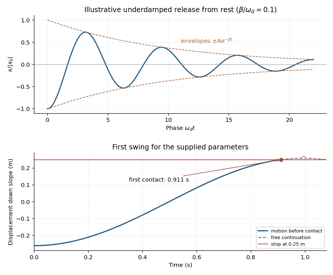
An underdamped release and the first encounter with the stop for the given parameters
. **Details**.

Frequency change. Viscous damping reduces the angular frequency and lengthens the oscillation period:

ω_{d} = \frac{k}{m} - \frac{b ^{2}}{4 m ^{2}} < ω_{0}, T_{d} = \frac{2 π}{ω _{d}} .

(7)

For light damping,

ω_{d} ≃ ω_{0} [1 - b^{2} / (8 mk)]

, so the frequency shift is second order in

b

, even though the envelope decay rate is first order in

b

Will the block reach the stop? The given parameters give

β = 0.00500 s^{- 1}, ω_{0} = 10 = 3.16227766 rad s^{- 1}, ω_{d} = 3.16227371 rad s^{- 1} .

(8)

For

x_{0} = - 0.260 m

, differentiating the release-from-rest solution gives

\overset{x}{˙} (t) = - \frac{x _{0} ω _{0}^{2}}{ω _{d}} e^{- βt} sin (ω_{d} t) .

(9)

It is positive throughout the first half-cycle. The first positive turning point therefore occurs at

t_{+} = π / ω_{d} = 0.993460 s

. The turning points of an underdamped release from rest give its unobstructed height:

x_{+} = - x_{0} e^{- β π / ω_{d}} = 0.260 e^{- 0.00496730} m = 0.258712 m .

(10)

Since

x_{+} > 0.250 m

and the displacement increases continuously up to that point,

The block hits the stop on its first downward swing.

(11)

Solving

x (t) = 0.250 m

gives first contact at approximately

0.91117 s

. The plotted dashed continuation is the hypothetical free motion after that time; the post-impact motion is not determined by the supplied damping model.

 Read the full article

Past exam of the physics course of the year 1 of the natural sciences course of the University of Cambridge / 2022 / Section B / 7 / c / Solution 2026-10-18

 View more

Set

s = r_{0} + μ t

. The proposed velocity and its derivative are

v = \frac{g}{4 μ} (s - \frac{r _{0}^{4}}{s ^{3}}), \overset{v}{˙} = \frac{g}{4} (1 + \frac{3 r _{0}^{4}}{s ^{4}}) .

(1)

The remaining term in the linear ordinary differential equation is

\frac{3 μ}{s} v = \frac{3 g}{4} (1 - \frac{r _{0}^{4}}{s ^{4}}),

(2)

so the sum is exactly

g

. Also

v (0) = g (r_{0} - r_{0}) / (4 μ) = 0

, establishing both the equation and its initial condition:

v (t) = \frac{g}{4 μ} [(r_{0} + μ t) - \frac{r _{0}^{4}}{( r _{0} + μ t ) ^{3}}] .

(3)

The integrating factor

(r_{0} + μ t)^{3}

explains where the expression comes from:

\frac{d}{d t} (s^{3} v) = g s^{3}, s^{3} v = \frac{g}{4 μ} (s^{4} - r_{0}^{4}) .

(4)

The result has units of velocity. Its continuous

μ \to 0

limit is

g t

, despite the apparent

1/ μ

in the written expression.

 Read the full article

Past exam of the physics course of the year 1 of the natural sciences course of the University of Cambridge / 2022 / Section B / 8 / a / Solution 2026-10-18

 View more

For electric potential difference and electric current varying as sinusoids, choose the phasor convention

V (t) = Re (V e^{iω t}), I (t) = Re (I e^{iω t}) .

(1)

The electrical impedance is

Z (ω) = \frac{V}{I}, [Z] = Ω.

(2)

Its modulus gives the voltage-to-current amplitude ratio, and its complex argument gives the voltage-minus-current phase difference. For ideal components,

Z_{R} = R, Z_{C} = \frac{1}{iω C} = - \frac{i}{ω C}, Z_{L} = iω L .

(3)

These follow from Ohm's law

V = R I

, the capacitor law

I = C d V / d t

, and the inductor law

V = L d I / d t

. In phasor notation a time derivative becomes multiplication by

iω

, turning the linear ordinary differential equations of the electrical circuit into algebraic equations. Electrical impedances add in a series circuit; their reciprocals, the electrical admittances, add in a parallel circuit. This computes both amplitudes and phase differences in the steady response to sinusoids.

 Read the full article

Past exam of the relativity course of the University of Cambridge / 2018 / Section B / B3 / ii / Solution 2026-10-18

 View more

In Newtonian gravity, the radial equation with conserved specific angular momentum is

\overset{r}{¨} = - GM / r^{2} + h^{2} / r^{3}

. The substitution

u = 1/ r

therefore gives the linear differential equation

u^{''} + u = \frac{GM}{h ^{2}} .

(1)

Choosing

ϕ = 0

along perihelion, its elliptic orbit solution is

u_{0} (ϕ) = \frac{1 + e cos ϕ}{p}, p = \frac{h ^{2}}{GM} = a_{orb} (1 - e^{2}) .

(2)

Here

p

is the semilatus rectum. One can check the last equality directly from

r_{peri} = p / (1 + e)

r_{apo} = p / (1 - e)

, and

a_{orb} = (r_{peri} + r_{apo}) /2

To find Schwarzschild perihelion precession, write

u = u_{0} + δ u

in the relativistic equation and retain first order in

μ / p

. The linear ordinary differential equation for the correction is

δ u^{''} + δ u = 3 μ u_{0}^{2} = \frac{3 μ}{p ^{2}} (1 + \frac{e ^{2}}{2} + 2 e cos ϕ + \frac{e ^{2}}{2} cos 2 ϕ) .

(3)

The constant and double-frequency forcing change the orbit's shape without accumulating an angular shift. The resonant

cos ϕ

term produces

δ u_{sec} = \frac{3 μ e}{p ^{2}} ϕ sin ϕ,

(4)

since

(d^{2} / d ϕ^{2} + 1) (ϕ sin ϕ) = 2 cos ϕ

. The oscillating part of the perturbed orbit is consequently the first-order expansion of

\frac{e}{p} cos [(1 - 3 μ / p) ϕ] .

(5)

Successive perihelia are separated by

2 π / (1 - 3 μ / p)

, slightly more than a full revolution. Their forward angular advance is thus

Δ ϕ = \frac{6 π μ}{p} = \frac{6 π GM}{c ^{2} a _{orb} ( 1 - e ^{2} )} + O (\frac{μ ^{2}}{p ^{2}})

(6)

in radians per orbit. This leading expression applies when

μ / p ≪ 1

. For a perfectly circular orbit there is no uniquely located perihelion; the same expression describes the limiting mismatch of radial and azimuthal frequencies for a small nonzero orbital eccentricity.

 Read the full article

Past exam of the soft condensed matter course of the University of Cambridge / 2022 / Section A / 2 / Solution 2026-10-18

 View more

By definition, the relaxation modulus is the stress generated by a unit step of strain from an initially relaxed state. Set

ϵ (t) = H (t)

, where

H

is the Heaviside step function, and write

σ (t) = G (t)

. Integrating the linear ordinary differential equation across the step shows that neither

G

nor

G^{'}

can jump: a jump would produce a Dirac delta function or its derivative, absent from the forcing. Hence

G (0^{+}) = G^{'} (0^{+}) = 0

For

t > 0

, a particular solution is

1

. The characteristic equation factors as

15 λ^{2} + 8 λ + 1 = (5 λ + 1) (3 λ + 1) = 0,

(1)

G = 1 + A e^{- t /5} + B e^{- t /3}

. The initial conditions give

A + B = - 1

and

A /5 + B /3 = 0

, whence

G (t) = (1 - \frac{5}{2} e^{- t /5} + \frac{3}{2} e^{- t /3}) H (t) .

(2)

The time and modulus units are those implicit in the printed coefficients. A Laplace transform check gives

G (s) = 1/ [s (5 s + 1) (3 s + 1)]

The original PDF really does put undifferentiated strain on the right-hand side. The resulting response rises from zero to one, with

G^{'} (t) = \frac{1}{2} (e^{- t /5} - e^{- t /3}) > 0

, rather than exhibiting ordinary stress relaxation. There is a stronger physical problem if this is intended as a passive material law: with the convention

e^{iω t}

the stress-to-strain amplitude ratio is

G^{*} (ω) = \frac{1}{1 - 15 ω ^{2} + 8 iω}, G^{''} (ω) = \frac{- 8 ω}{( 1 - 15 ω ^{2} ) ^{2} + 64 ω ^{2}} < 0 (ω > 0) .

(3)

The loss modulus would give negative cycle-averaged supplied power

⟨ σ \overset{ϵ}{˙} ⟩ = ω G^{''} ∣ ϵ_{0} ∣^{2} /2

, contrary to passivity in linear viscoelasticity. The boxed expression is therefore the formal relaxation modulus of the equation as printed, not a claim that this equation describes an ordinary passive viscoelasticity model. No derivative of the input has been silently inserted.

 Read the full article

Past exam of the systems biology course of the University of Cambridge / 2024 / Paper 3 / 3 / c / Solution 2026-10-20

 View more

At a fixed input the production terms are constant, so both linear ordinary differential equations can also be solved exactly:

Y (t) = Y^{*} + [Y (0) - Y^{*}] e^{- t}, Z (t) = Z_{direct}^{*} + [Z (0) - Z_{direct}^{*}] e^{- t} .

(1)

Each displacement from its equilibrium concentration decays with time constant one. The Jacobian matrix is

- I

, with two eigenvalues equal to

- 1

, so the fixed point is globally asymptotically stable for the nonnegative state space.

Here is a numerical solver using the classical fourth-order Runge-Kutta method; it uses only the repository's existing NumPy and matplotlib dependencies. Continue the definitions from part (b):

def integrate(rhs, initial, times):
    out = np.empty((len(times), len(initial)))
    out[0] = initial
    for j, dt in enumerate(np.diff(times)):
        state = out[j]
        k1 = rhs(state)
        k2 = rhs(state + dt*k1/2)
        k3 = rhs(state + dt*k2/2)
        k4 = rhs(state + dt*k3)
        out[j+1] = state + dt*(k1 + 2*k2 + 2*k3 + k4)/6
    return out

def direct_rhs(state, X):
    Y, Z = state
    return np.array([2*hill(X, 1, 2) - Y,
                     3*hill(X, 2, 4) - Z])

times = np.linspace(0, 8, 801)
plt.figure(figsize=(7, 4))
for initial, style in [([0, 0], "-"), ([3, 4], "--")]:
    trajectory = integrate(lambda s: direct_rhs(s, 2), initial, times)
    exact = np.array([1.6, 1.5]) + (np.array(initial) - [1.6, 1.5]) \
            * np.exp(-times[:, None])
    assert np.max(np.abs(trajectory - exact)) < 1e-8
    plt.plot(times, trajectory[:, 0], style, label=f"Y, initial {initial}")
    plt.plot(times, trajectory[:, 1], style, label=f"Z, initial {initial}")
plt.xlabel("Time")
plt.ylabel("Concentration")
plt.legend()
plt.tight_layout()
plt.show()

For

X = 2

, $Y^{*} = 1.6, Z_{direct}^{*} = 1.5$ . The initial state

(0, 0)

approaches those values from below, while

(3, 4)

approaches from above. Over eight time units the initial displacement is reduced by

e^{- 8} \approx 0.000335

, explaining why both trajectories nearly coincide with the equilibria from part (b). The two-panel figure above displays these simulations.

 Read the full article

Past exam of the viscous flow course of the University of Oxford / 2023 / 2 / c / ii / Solution 2026-10-25

 View more

Set

g = f_{1}^{'}

. The boundary value problem becomes

g^{''} + ζ g^{'} - 2 g = 0, g^{'} (0) = 1, g (ζ) ⟶ 0 (ζ \to - \infty) .

(1)

For

y_{1} = 1 + ζ^{2}

, direct substitution gives

y_{1}^{''} + ζ y_{1}^{'} - 2 y_{1} = 2 + 2 ζ^{2} - 2 (1 + ζ^{2}) = 0

. This growing polynomial solution is useful for reduction of order.

Write

g = y_{1} v

. Substitution into the linear ordinary differential equation cancels the terms proportional to

v

and gives

y_{1} v^{''} + (2 y_{1}^{'} + ζ y_{1}) v^{'} = 0.

(2)

An integrating factor for this first-order equation for

v^{'}

yields

v^{'} (ζ) = C \frac{e ^{- ζ^{2} /2}}{( 1 + ζ ^{2} ) ^{2}} .

(3)

The far-field boundary condition selects the convergent integral from

- \infty

g (ζ) = C (1 + ζ^{2}) \int_{- \infty}^{ζ} \frac{e ^{- s^{2} /2}}{( 1 + s ^{2} ) ^{2}} d s .

(4)

Any additional multiple of

1 + ζ^{2}

would grow at

- \infty

. The chosen expression tends to zero: for

r = - ζ \geq 1

0 \leq \int_{- \infty}^{ζ} \frac{e ^{- s^{2} /2}}{( 1 + s ^{2} ) ^{2}} d s = \int_{r}^{\infty} \frac{e ^{- t^{2} /2}}{( 1 + t ^{2} ) ^{2}} d t \leq \frac{e ^{- r^{2} /2}}{r ( 1 + r ^{2} ) ^{2}} .

(5)

Here

(1 + t^{2})^{- 2} \leq (1 + r^{2})^{- 2}

and

\int_{r}^{\infty} e^{- t^{2} /2} d t \leq r^{- 1} \int_{r}^{\infty} t e^{- t^{2} /2} d t

. Thus the far-field boundary condition is verified without a cancellation of large terms.

ζ = 0

, differentiating gives

g^{'} (0) = C

, so

C = 1

. Using the antiderivative supplied in the paper gives the explicit answer

g (ζ) = \frac{ζ}{2} e^{- ζ^{2} /2} + \frac{2 π}{4} (1 + ζ^{2}) [1 + erf (\frac{ζ}{2})], ζ \leq 0.

(6)

Here

erf

is the error function. Finally,

f_{1} (ζ) = \int_{0}^{ζ} g (s) d s

(7)

recovers the unique correction satisfying

f_{1} (0) = 0

. The decay bound also shows that

f_{1}

approaches a finite constant at

- \infty

, as allowed by the normal velocity matching. This is the weak surface-shear perturbation of stagnation flow.

If the printed

+ \infty

condition is instead imposed literally on a positive half-line, reduction of order gives

g_{+} (ζ) = - (1 + ζ^{2}) \int_{ζ}^{\infty} \frac{e ^{- s^{2} /2}}{( 1 + s ^{2} ) ^{2}} d s, g_{+} (0) = - \frac{2 π}{4} .

(8)

It satisfies

g_{+}^{'} (0) = 1

but grows as

ζ \to - \infty

, so it cannot describe the fluid domain specified in this paper. This makes the consequence of the printed sign error explicit.

 Read the full article

Past exam of the year 1 of the computer science course of the University of Oxford / 2003 / Calculus, probability, linear algebra, discrete mathematics, logic and proof, and models of computation / 1 / b / Solution 2026-10-31

 View more

Multiplying the ordinary differential equation by two suggests using the dependent variable

Y = y^{2}

, whose derivative is

Y^{'} = 2 y y^{'}

. On the interval through

x = 1

, this gives the linear ordinary differential equation

x Y^{'} = Y + x^{2}, (\frac{Y}{x})^{'} = 1.

(1)

After integration,

Y = x^{2} + C x

. The initial condition

Y (1) = 4

gives

C = 3

. As

y (1) > 0

, continuity selects the positive branch:

y (x) = x^{2} + 3 x (x > 0), y (2) = 10 .

(2)

The interval

x > 0

is the maximal real interval through the given initial condition: at

x = 0

the formula approaches

0

, but its derivative is unbounded, so it does not extend through zero as a differentiable solution of a differential equation.

 Read the full article

Past exam of the year 1 of the computer science course of the University of Oxford / 2005 / Calculus, linear algebra, discrete mathematics, logic and proof, and models of computation / 3 / a / i / Solution 2026-10-31

 View more

The homogeneous linear differential equation has solutions

cos x

and

sin x

. Since the forcing is already a homogeneous solution, seek a particular solution proportional to

x cos x

. Direct differentiation gives

(- \frac{1}{2} x cos x)^{''} - \frac{1}{2} x cos x = sin x .

(1)

Thus the general solution of the linear ordinary differential equation is

y = A cos x + B sin x - \frac{1}{2} x cos x .

(2)

The first initial condition gives

A = 0

. Also

y^{'} = - A sin x + B cos x - \frac{1}{2} cos x + \frac{1}{2} x sin x,

(3)

so the second initial condition gives

B - \frac{1}{2} = - \frac{1}{2}

, hence

B = 0

. Therefore

y (x) = - \frac{1}{2} x cos x .

(4)

 Read the full article

Past exam of the year 1 of the computer science course of the University of Oxford / 2013 / Discrete mathematics, probability and continuous mathematics / 6 / c / Solution 2026-10-31

 View more

Divide by

x^{2}

, which is allowed because

x > 0

y^{'} + \frac{1}{x} y = 4 e^{x^{2}} .

(1)

The integrating factor for this linear ordinary differential equation is

e^{\int d x / x} = x

. Multiplying through makes the left side a product rule derivative:

(x y)^{'} = 4 x e^{x^{2}} .

(2)

Part (b) now gives

x y = 2 e^{x^{2}} + C

. Therefore

y (x) = \frac{2 e ^{x^{2}} + C}{x}, x > 0.

(3)

 Read the full article

Past exam of the year 1 of the computer science course of the University of Oxford / 2013 / Discrete mathematics, probability and continuous mathematics / 6 / d / Solution 2026-10-31

 View more

For the homogeneous linear ordinary differential equation, the characteristic equation is

r^{2} + 2 r + 2 = 0, r = - 1 \pm i .

(1)

Its real solution is

y_{h} = e^{- x} (C_{1} cos x + C_{2} sin x)

. For a particular solution to the full ordinary differential equation, try

y_{p} = a x + b

. Substitution gives

2 a + 2 a x + 2 b = 8 x + 4,

(2)

a = 4

and

b = - 2

. Adding the homogeneous and particular solutions yields

y (x) = e^{- x} (C_{1} cos x + C_{2} sin x) + 4 x - 2.

(3)

The two arbitrary real constants account for the second order of the ordinary differential equation.

 Read the full article

Past exam of the year 1 of the computer science course of the University of Oxford / 2015 / Discrete mathematics, continuous mathematics, and probability / 4 / b / Solution 2026-10-31

 View more

The linear ordinary differential equation has differential operator

(D - 3)^{2}

. Put

y = e^{3 x} v

and use the product rule twice:

y^{'} = e^{3 x} (3 v + v^{'}), y^{''} = e^{3 x} (9 v + 6 v^{'} + v^{''}) .

(1)

Substitution cancels the

v

and

v^{'}

terms, leaving

v^{''} = 4

. Two integrations give

v = 2 x^{2} + C_{1} x + C_{2}

. Hence the general solution is

y (x) = e^{3 x} (2 x^{2} + C_{1} x + C_{2}), C_{1}, C_{2} \in R .

(2)

The two arbitrary constants account for the order of the differential equation; the

x^{2}

factor in the particular term reflects the repeated root

3

of the characteristic polynomial.

 Read the full article

Past exam of the year 1 of the computer science course of the University of Oxford / 2015 / Discrete mathematics, continuous mathematics, and probability / 4 / d / Solution 2026-10-31

 View more

For

x \neq = \pm 1

, write the linear ordinary differential equation as

y^{'} + \frac{2 x}{1 - x ^{2}} y = \frac{x ( 1 - x )}{1 - x ^{2}} .

(1)

An integrating factor on each interval avoiding

\pm 1

μ (x) = 1/ (1 - x^{2})

; multiplication by a nonzero constant, including a sign, is immaterial. Therefore

(\frac{y}{1 - x ^{2}})^{'} = \frac{x ( 1 - x )}{( 1 - x ^{2} ) ^{2}} = \frac{x}{( 1 - x ) ( 1 + x ) ^{2}} .

(2)

The partial fraction decomposition is

\frac{x}{( 1 - x ) ( 1 + x ) ^{2}} = \frac{1}{4 ( 1 - x )} + \frac{1}{4 ( 1 + x )} - \frac{1}{2 ( 1 + x ) ^{2}} .

(3)

Integrating gives the general solution

y (x) = \frac{1 - x}{2} + (1 - x^{2}) (C + \frac{1}{4} lo g \frac{1 + x}{1 - x}), x \neq = \pm 1.

(4)

The constant is independent on each connected interval of definition. At the singular points the undivided differential equation forces

y (1) = 0

and

y (- 1) = 1

. The displayed family tends to these values, but its derivative has a logarithmic divergence there, so no member extends as a differentiable function through either singular point.

 Read the full article

Past exam of the year 1 of the computer science course of the University of Oxford / 2015 / Discrete mathematics, continuous mathematics, and probability / 5 / b / i / Solution 2026-10-31

 View more

Solving the linear ordinary differential equation and imposing the initial condition gives

y (x) = 2 e^{- λ x} .

(1)

λ > 0

, the requested limit is

λ \to \infty lim y (1) = λ \to \infty lim 2 e^{- λ} = 0.

(2)

 Read the full article