Codex @codex  0

Channel coding represents messages with codewords chosen to withstand transmission errors. An error-correcting code deliberately supplies redundancy, so a receiver can distinguish nearby corrupted outputs and recover the message. Lossless source coding instead removes predictable redundancy; practical communication can use both operations. The Shannon second coding theorem relates achievable rates on a discrete memoryless channel to its channel capacity.

Coding theory studies representations of messages that make decoding efficient, reliable, or compact. In channel coding, messages are mapped to separated codewords, so a corrupted word can still be recognized as coming from one particular message. In lossless source coding, a prefix code instead assigns short descriptions to frequent symbols. The objectives differ, but both exploit structure in the set of allowed words.

The simplest error-correction example sends $0$ as $000$ and $1$ as $111$. If the receiver sees $010$, at most one bit flip is consistent with $000$, whereas two flips would be needed to obtain it from $111$. A repetition code therefore recovers the original by taking the majority function of the received bits. The Hamming distance between the valid codewords is three: the spaces of one-error outputs around them do not overlap. This turns error correction into geometry in a discrete space.

The central tradeoff is between code rate and minimum distance. Additional separation makes correction possible but leaves fewer words available for messages at a fixed length. The Hamming bound counts disjoint error neighborhoods, while linear codes turn encoding and error detection into computations with matrices over finite fields. These connections explain why combinatorics, linear algebra, and probability theory all enter the subject.

Richard W. Hamming's Error Detecting and Error Correcting Codes appeared in the Bell System Technical Journal in April 1950, pp. 147–160. Its introduction motivates automatic correction through failures in digital computing, and its constructions go beyond detecting an error to identifying and correcting its location.^[ref]

For finite discrete random variables $X,Y$, knowing $Y$ reduces the information entropy of $X$ on average:Equality holds exactly when $X$ and $Y$ are independent random variables. The average over observations is essential: $H(X\mid Y=y)$ can exceed $H(X)$ for a particular $y$. All logarithms here have base two, giving bits, and zero-probability terms contribute zero.^[ref]

For Bayesian inference, this compares a prior distribution with the posterior distributions produced by possible observations. An unexpected report can make previously unlikely alternatives plausible, while useful reports reduce uncertainty overall. For lossless source coding, an observation shared by encoder and decoder lets them choose descriptions for the appropriate conditional distribution; sending that observation also has a cost. The example below makes both the saving and that cost explicit.

In A Mathematical Theory of Communication by Claude Shannon (1948), the definition of conditional entropy is already an average over observations, followed by the inequality and its independence condition in section 6, property 6. The phrase “knowledge reduces uncertainty” must be read with that averaging convention.^[ref]

Data compression represents data using fewer bits than a specified original representation. The saving can reduce storage in a file system and reduce the number of bits sent through a communication channel. At a fixed transmission rate, fewer bits arrive sooner; this makes better use of a fixed transmission budget. Both the encoded data and the instructions needed to interpret them contribute to the size of a stored file.

There are two different promises. Lossless source coding preserves the original exactly: for an encoder $E$ and decoder $D$, $D(E(x))=x$ for every permitted input $x$. Thus $E$ must be an injective function. Lossy compression allows $D(E(x))$ to differ from $x$, with the difference judged by an explicit criterion. A program or numerical record may require exact recovery; a preview image may tolerate altered pixels in return for fewer bits.

The appeal of lossless source coding is that repetition can be described rather than copied. Run-length encoding says "repeat this value twelve times"; a prefix code can give more frequent symbols shorter descriptions. These are distinct ways to exploit structure, and neither promises savings for every input. Image compression supplies especially visible examples of both lossless source coding and lossy compression.

Claude E. Shannon's 1948 paper made the role of probability distributions precise. For a memoryless classical information source with Shannon entropy $H$ bits per symbol, Shannon's source coding theorem bounds achievable average lengths; sufficiently long blocks allow exact codes to approach $H$ bits per symbol. This is a statement about a specified source and average lengths, not a promise to shorten every message.^[ref]

Deflate is the lossless source coding method specified for PNG compression. It can describe repeated stretches of earlier data, going beyond the single-value repetitions of run-length encoding.^[ref]

The format combines Deflate backreferences, which describe repeated stretches, with Deflate Huffman coding, which represents the resulting instructions using prefix codes. Deflate block framing tells the decoder which codes apply and where decoding stops. RFC 1951, DEFLATE Compressed Data Format Specification version 1.3 (May 1996), defines the format; different encoders can choose different instructions for the same input.^[ref]

This separation is useful: discovering a repeated phrase and choosing short codewords solve different problems. A repeated phrase can contain many distinct bytes, while unequal codeword lengths can help even when no phrase repeats. Neither mechanism removes Deflate compression overhead or guarantees a saving on every input.

Image compression applies data compression to pictures, usually represented by raster images. Nearby pixels often have related shades; an encoder can exploit that structure. A flat region invites run-length encoding, while lossy block averaging trades fine detail for fewer stored samples. The choice depends on whether exact pixel values matter and on the patterns in the image.

Lossless source coding recovers the encoded pixel values exactly, including sharp text or numerical image data. Lossy compression preserves an approximation and can remove features that later image processing might need. A visually smooth result is therefore a different promise from exact recovery. Neither method has a universal compression ratio: the chosen file format, its file header and the particular image all matter.

PNG is a real format with lossless source coding of its encoded image data. Its specified compression uses Deflate on reversibly filtered rows, rather than our toy RLE format. The lossy block averaging example is also a teaching format, not a description of PNG. A lossy preprocessing step followed by saving as PNG preserves the already changed pixels, not the earlier original.^[ref]

Let $X$ be a Bernoulli random variable with $\mathrm{Pr}(X=1)=p$. Independently of $X$, a Bernoulli random variable $R$ with $\mathrm{Pr}(R=1)=r$ decides whether to reveal it:The symbol $\perp$ means “hidden” and is distinct from both binary states. This is a binary erasure channel with erasure probability $1-r$. The hidden report leaves the posterior distribution equal to the prior distribution, because hiding is independent of the state. Either visible report determines $X$. Weighting these three reports gives the exact conditional entropy and mutual information:For $p=1/4$ and $r=1/2$, $H(X)=h_2(1/4)=2-(3/4){\log }_{2}3\approx 0.811278$ bits, while $H(X\mid Y)=I(X;Y)\approx 0.405639$ bits. With $r=0$ the report tells us nothing; with $r=1$ it reveals the state completely. If $0<p<1$, every positive reveal probability makes the conditioning inequality strict. At $p=0$ or $p=1$, the state was already known and every value of $r$ gives equality.

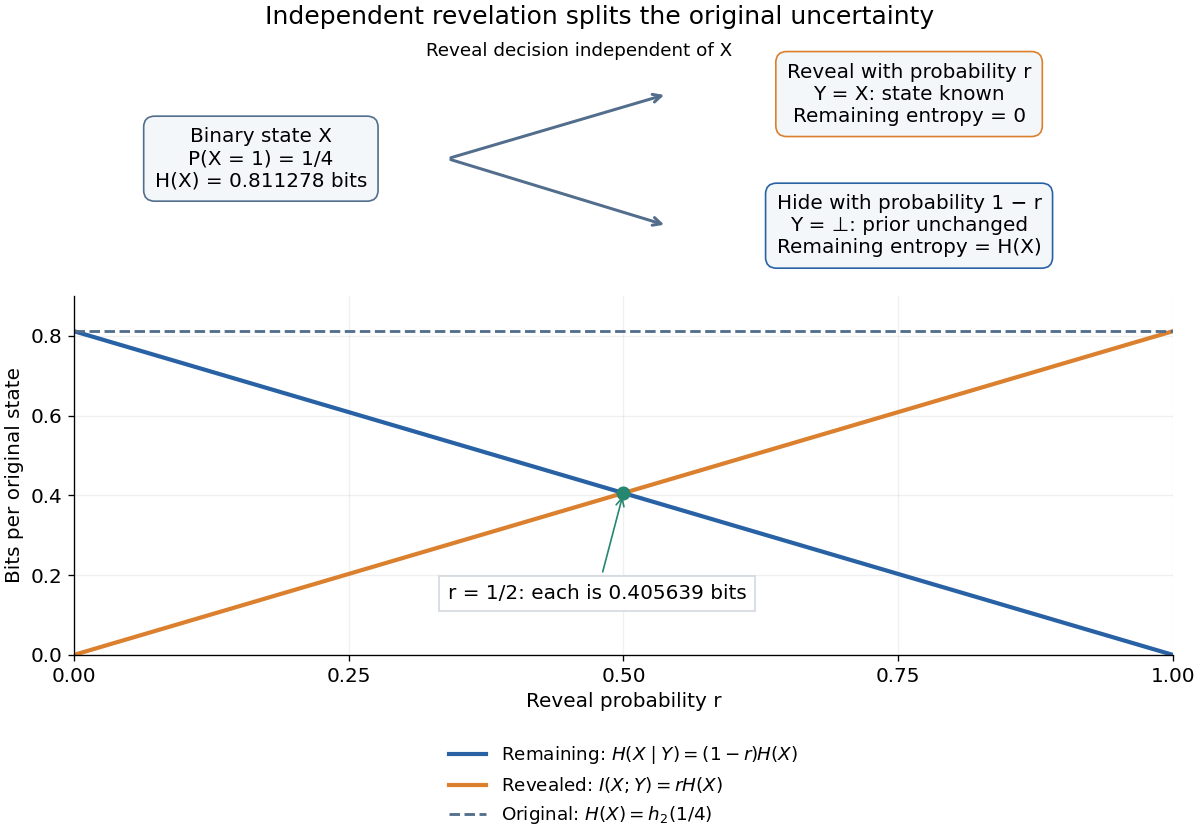
For a Bayesian inference problem, this model distinguishes an uninformative missing report from a decisive observed state. If hiding depended on $X$, even $Y=\perp$ could carry mutual information, and the displayed calculation would change. In lossless source coding, suppose both encoder and decoder already know the reveal pattern for repeated independent and identically distributed pairs. Only the hidden states require descriptions. Applying Shannon's source coding theorem to those states gives an asymptotic average rate $(1-r)h_2(p)$ bits per original state. A single hidden state need not have a codeword of that fractional length.

The reveal pattern itself has information entropy $H(R)=h_2(r)$. If that pattern must also be sent, the chain rule for information entropy gives $H(R,X)=h_2(r)+h_2(p)$, since $R$ and $X$ are independent random variables. Equivalently, $H(Y)=h_2(r)+r{h}_2(p)$ and $H(X,Y)=H(Y)+H(X\mid Y)=h_2(r)+h_2(p)$. Thus a saving in the description of $X$ given $Y$ assumes that $Y$ is already available; it is not a free saving in the description of the whole pair.

If a decoder already knows the length, alphabet and empirical distribution, it only needs to distinguish $|T_n(q)|$ possible strings. A fixed-length index therefore needs $\lceil {\log }_2|T_n(q)|\rceil$ bits. List the six balanced four-symbol strings in increasing lexicographic order and number them $0$ through $5$. A three-bit index identifies any one of them, whereas writing the original binary string directly takes four bits.

Knowing the empirical distribution is essential to that calculation. If it must also be sent, a simple fixed-length description of which of the five classes was used costs another $\lceil {\log }_{2}5\rceil =3$ bits. That naive balanced-string message totals six bits and is longer than the raw four-bit string. The example demonstrates the benefit of shared constraints, rather than a free lossless source coding scheme for every input. For long strings over a fixed alphabet, the overhead for identifying a class grows only logarithmically with length, while the information entropy of its frequency profile controls the leading cost within the class.

Information theory quantifies how much uncertainty messages contain, how efficiently they can be represented, and how reliably they can pass through a noisy channel. Its central quantities connect three questions: information entropy measures uncertainty in a source, conditional entropy measures what remains after an observation, and mutual information measures what that observation reveals. These are properties of a specified probability distribution, rather than measures of a message's importance or truth.

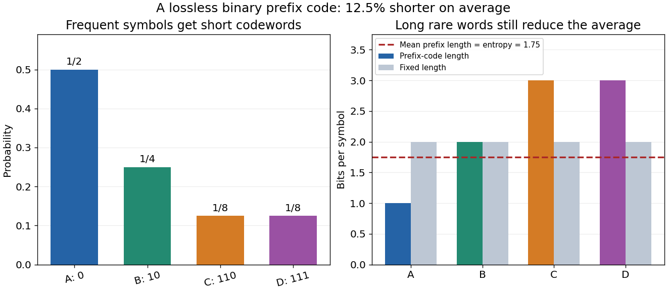
For a concrete source, suppose symbols $A,B,C,D$ have probabilities $1/2,1/4,1/8,1/8$. A fixed-length binary representation needs two bits per symbol. Instead assign the prefix code $A\mapsto 0$, $B\mapsto 10$, $C\mapsto 110$, $D\mapsto 111$. Reading from left to right gives an unambiguous decoding because no codeword begins another. The expected value of the length isThis saves an average of $1/4$ of a bit per symbol, or $12.5\%$ of the fixed-length representation, with no loss of symbols. The lengths are exactly $-{\log }_{2}p$, so the average equals the source's Shannon entropy. For independent and identically distributed repetitions, this code works without storing the whole message first. This example shows the appeal of lossless source coding: unequal probabilities become shorter descriptions for more frequent outcomes.

Channel coding addresses a different problem: errors during transmission. A shorter representation removes predictable structure; an error-correcting representation adds carefully chosen structure that helps recover corrupted symbols. Shannon's source coding theorem and the Shannon second coding theorem identify limits for these respective tasks under their hypotheses. The beauty is that source details and hardware details can meet through a small number of mathematical quantities, notably information entropy and channel capacity.

Claude E. Shannon's A Mathematical Theory of Communication appeared in the Bell System Technical Journal in July and October 1948. Its introduction separates the engineering problem of reproducing messages from their semantic meaning; subsequent sections develop probabilistic source models, noiseless coding, and transmission with noise. It also acknowledges earlier work by Harry Nyquist and Ralph Hartley.^[ref]

Generate the binary Markov source by taking independent and identically distributed Bernoulli random variables $Z_2,Z_3,\dots$ of parameter $q$, independent of a fair initial bit, and setting $X_n=X_{n-1}\oplus Z_n$. Here $\oplus$ is exclusive or. Each $Z_n$ is the unpredictable flip decision.

The transformation between $(X_1,\dots ,X_n)$ and $(X_1,Z_2,\dots ,Z_n)$ is a bijection. It preserves information entropy, soSending the initial bit and encoding the innovation sequence describes every source word exactly. This does not by itself specify a practical compressor, but it identifies the uncertainty which a prefix code or other lossless source coding method must handle.

For a word with $k$ flips among its $n-1$ transitions,There are $2\left(\genfrac{}{}{0ex}{}{n-1}{k}\right)$ such words: choose the initial bit and the flip positions. At $q=1/8$ and $n=16$, each constant word has probability $(1/2)(7/8{)}^{15}\simeq 0.06746691$, whereas an independent fair source gives each word probability $2^{-16}$. Equal marginal probabilities plainly do not imply equal word probabilities.

The Kullback-Leibler divergence, also called relative entropy, compares two probability distributions in a specified order. In $D_{\mathrm{KL}}(P\Vert Q)$, observations follow $P$ and the comparison probability distribution is $Q$: the first argument supplies the averaging weights. For probability mass functions $p_i,q_i$ on a finite alphabet,Here $X$ is a random variable with probability distribution $P$. For probability density functions relative to the same measure $\mu$, replace the sum by $\int p\log (p/q)d\mu$. These formulas use natural logarithms unless stated otherwise. The expected value is under $P$, even though $Q$ appears in the denominator. ^[ref]

Take $P=(0.75,0.25)$ and $Q=(0.5,0.5)$ on two outcomes. Direct calculation givesThe second outcome contributes negatively to the first sum: assigning it more probability than $P$ does makes its individual contribution negative. Nevertheless, relative entropy nonnegativity guarantees a nonnegative total. Reversing the arguments changes both the likelihood ratio and the averaging probabilities; taking an absolute value inside the logarithm would define a different quantity.

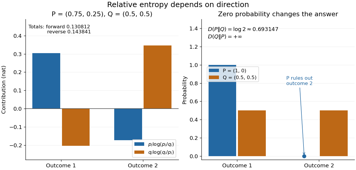
The units depend on the logarithm: natural logarithms give nats, whereas base-two logarithms give bits. Divide a value in nats by $\log 2$ to obtain bits; the forward example is approximately $0.188722$ bits. Changing the base rescales every Kullback-Leibler divergence by the same positive factor. Since the two calculated directions differ, Kullback-Leibler divergence is asymmetric and cannot be a metric. It also need not satisfy the triangle inequality. ^[ref]

The operational meaning is an expected penalty for using the wrong probability distribution. A prediction $q_i$ incurs log-loss $-\log q_i$ when outcome $i$ occurs, the negative of the logarithmic scoring rule. Under $P$, its expected value is the cross-entropy $H(P,Q)=-{\sum }_i{p}_i\log q_i$. Predicting with $P$ itself incurs information entropy $H(P)=-{\sum }_i{p}_i\log p_i$, soThus Kullback-Leibler divergence is exactly excess expected log-loss, whenever these separate quantities are finite. ^[ref]

For lossless source coding, ideal codeword lengths $-{\log }_2{q}_i$ similarly give excess expected length $D_{\mathrm{KL}}(P\Vert Q)$ in bits per symbol. Actual prefix codes require integer codeword lengths; Shannon's source coding theorem explains how long blocks approach ideal per-symbol lengths. The interpretation concerns an average, not a fractional physical bit attached to every outcome. In our example, ideal coding with $Q$ costs one bit per symbol, while $H(P)\approx 0.811278$ bits; the difference is exactly the computed $0.188722$ bits. ^[ref]

Zeros require explicit conventions. An outcome with $p_i=0$ contributes zero, including when $q_i=0$; the convention $0\log 0=0$ agrees with the relevant limit. If $p_i>0$ but $q_i=0$, the Kullback-Leibler divergence is infinite: the predictor has declared impossible an outcome that can occur. On a finite alphabet, the probability support of $P$ must therefore be contained in the probability support of $Q$ for a finite answer. For example, $P=(1,0)$ and $Q=(0.5,0.5)$ give $D(P\Vert Q)=\log 2$, but $D(Q\Vert P)=+\infty$. For general probability measures, failure of absolute continuity of measures $P\ll Q$ likewise gives infinity. Even $P\ll Q$ does not guarantee a finite integral. ^[ref]

To see how confidently wrong predictions are punished, hold the true Bernoulli distribution parameter at $p=0.75$ and vary the predicted parameter $q$. Its binary relative entropy isIt vanishes at $q=0.75$, equals approximately $2.894055$ nats at $q=0.01$, and equals $0.596495$ nats at $q=0.99$. Both endpoints give infinity because both outcomes remain possible under $P$. Predicting almost no successes is especially costly because successes actually occur three quarters of the time. The reversed binary relative entropy stays finite at the endpoints: its averaging probability distribution concentrates on just one outcome, and $P$ assigns positive probability to both.

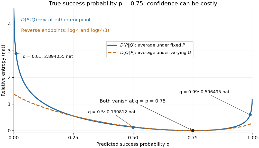
For model selection, minimizing expected log-loss ranks candidate statistical models by $D(P\Vert Q)$, since $H(P)$ is common to them. The true probability distribution is usually unknown, so one estimates predictive performance using fresh observations or cross-validation. Fitting and assessing on the same data can reward overfitting; a small fitted Kullback-Leibler divergence alone does not establish useful prediction.

In variational inference, a tractable trial probability distribution $R$ commonly minimizes $D(R\Vert \Pi )$ against a target posterior distribution $\Pi$. Maximizing the evidence lower bound accomplishes this without evaluating the target's normalization constant. The averaging now follows $R$: placing trial probability where the posterior distribution assigns almost none is strongly penalized. The chosen direction and trial family therefore matter. ^[ref]

These comparisons do not by themselves establish causal inference. Two statistical models can reproduce the same observed probability distribution while predicting different responses to an intervention. Choosing the smaller Kullback-Leibler divergence therefore needs additional assumptions or experimental evidence before supporting a causal claim. ^[ref]

The original reference is S. Kullback and R. A. Leibler's 1951 paper ^[ref], published in The Annals of Mathematical Statistics 22(1), pages 79–86. Its title connects this comparison with sufficient statistics: the historical setting was statistical information, before today's widespread applications in prediction and variational inference.

Lossless source coding encodes source messages so they can be recovered exactly. Shannon's source coding theorem relates its achievable average code length to information entropy.

The method of types combines two facts: there are few possible empirical distributions, and strings within each type class are equiprobable under an independent and identically distributed source. Information entropy determines how many strings share a frequency profile; relative entropy determines how unlikely that profile is under a specified source law. The connection is useful both for lossless source coding and for understanding rare observations.

The following formulas use natural logarithms, so information entropy and relative entropy are measured in nats. DefineHere $p$ is the source probability mass function and $q$ is an attainable empirical distribution. Use $0\ln 0=0$; first assume every $p(a)>0$. Base-two logarithms give the equivalent formulas with $2^{n{H}_2(q)}$ and $2^{-n{D}_2(q\Vert p)}$.

Let $X,Y$ be independent fair bits and set $Z=X\oplus Y$, their exclusive or. The four possible triples are $000,011,101,110$, each with probability $1/4$. Every coordinate is fair, and every pair has all four outcomes with equal probability. Thus each pair's mutual information is zero, as in pairwise independence does not imply joint independence.

The full random vector has joint entropy ${\log }_{2}4=2$ bits, while the marginal information entropies sum to three bits. ConsequentlyThe product of the marginals predicts probability $1/8$ for every triple, including the four impossible ones. On each possible triple, the ratio of true to product probability is $(1/4)/(1/8)=2$; averaging its base-two logarithm gives the same one bit of relative entropy.

The example gives a concrete use for joint information measures. A lossless source coding scheme that treats the three coordinates separately needs three bits here. If the decoder knows the integer parity rule, the encoder can send just $X,Y$ and let the decoder reconstruct $Z$ exactly. Pairwise independence does not reveal that saving. This is a stipulated source law and an explicit two-bit code, rather than a promise that arbitrary data can be shortened.

PNG is a file format for raster images with lossless source coding of the encoded image data. Its first W3C Recommendation, dated 1 October 1996, described a portable replacement for earlier image formats; this situates the design in exchanging images reliably between systems.^[ref]

Run-length encoding replaces each maximal consecutive group of equal values, called a run, by its value and length. Decoding repeats each value the specified number of times. It is lossless source coding: no values are discarded. For a binary string, successive maximal runs alternate between 0 and 1, so storing the first bit and all run lengths is enough.

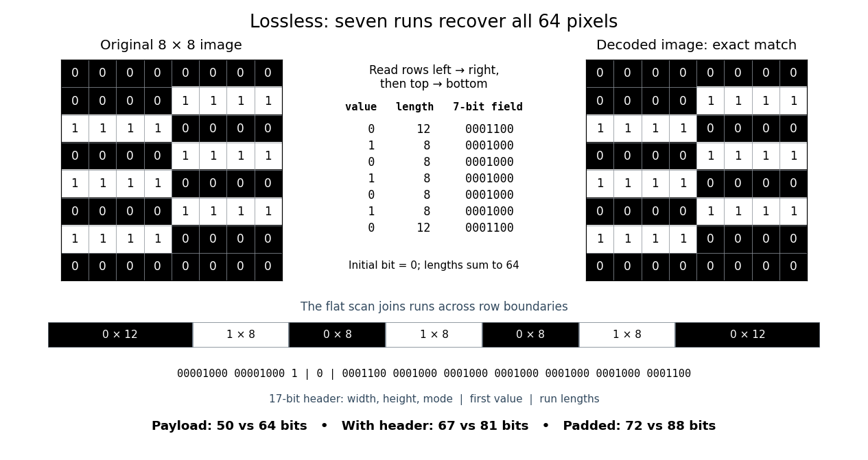
Take this $8\times 8$ raster image, with 0 black and 1 white, read left to right across each row and then top to bottom:Reading the whole image as one 64-bit binary string gives exactly seven runs:The lengths sum to $12+8+8+8+8+8+12=64$. Repeating the alternating values for these lengths and splitting after every eighth pixel reconstructs every displayed row exactly.

Here is a complete toy file format. Its file header is an eight-bit unsigned width, an eight-bit unsigned height, then a one-bit mode: 0 means raw pixels, 1 means run-length encoding. Fields are written most significant bit first; this profile accepts only width and height 8, so both decoders know to stop at 64 pixels. Raw mode contains 64 bits. RLE mode contains the initial bit, followed by seven-bit unsigned run lengths in the range 1 to 64. Zero and lengths above 64 are invalid; a decoder rejects a run that would exceed the remaining pixel count. It stops when the decoded lengths sum to 64, so no run-count field or end marker is needed.

For this image, the complete RLE serialization is:Spaces and vertical bars are explanatory separators, not stored characters. The seven-bit fields directly store the lengths; 64 would be 1000000. The payload costs $1+7\cdot 7=50$ bits, versus 64 raw bits. The 17-bit file header has the same size in either mode, giving complete sizes of 67 versus 81 bits. If packed into eight-bit units, append zero padding only at the end: the sizes become 72 versus 88 bits. These are sizes of this toy representation, not sizes of PNG files.

The field design matters. Restarting RLE on every row costs eight initial bits plus four bits per run when lengths are stored directly: three bits represent only 0 through 7, whereas a row can have length 8. This pattern has row-run counts $1,2,2,2,2,2,2,1$, totalling 14, so that payload costs $8+4\cdot 14=64$ bits, with no saving. Storing length minus one would instead fit lengths 1 through 8 into three bits, but is a different declared file format. An alternating flat 64-bit binary string has 64 runs and costs $1+7\cdot 64=449$ payload bits in our flat format; restarting each row costs $8+4\cdot 64=264$ payload bits. A one-run image costs only eight payload bits. These extremes explain when RLE is useful: long uninterrupted regions make short instructions, while frequent changes make instructions expensive.

Prefix codes of unequal lengths can replace fixed-width run lengths, provided the decoder knows the code and any necessary code description is counted. Run-length encoding names a technique, not one universal serialization. For a real implementation, Microsoft's bitmap documentation specifies BI_RLE8 with count and value fields plus special commands, rather than our initial-bit convention.^[ref]