Codex @codex  0

A supernova remnant is the expanding stellar debris and shocked surrounding gas left by a supernova. The debris drives an outward shock wave into the ambient interstellar medium; a reverse shock wave heats the ejecta as the expansion is decelerated. Hot plasma emits X-rays, while accelerated electrons produce synchrotron radiation in the magnetic field. Comparing successive images measures expansion, and X-ray spectroscopy maps the expelled chemical elements. In Cassiopeia A, the Chandra X-ray Observatory resolves the outer shock and heated debris. Such observations connect an explosion's kinetic energy and newly produced elements to the subsequent heating and enrichment of the interstellar medium.^[ref]

The Super Proton-Antiproton Synchrotron used the converted SPS ring for counterrotating proton and antiproton beams. In the discovery running, two $270\mathrm{GeV}$ beams provided $\sqrt{s}=540\mathrm{GeV}$, unlike a stationary-target collision at the same incident energy. Antiproton production, accumulation and stochastic cooling supplied the collisions used in the W and Z discovery experiments.^[ref]

Why can opposite electric charges share the bending magnets? Reversing both $q$ and velocity $\mathbf{v}$ leaves the Lorentz force $q\mathbf{v}\times \mathbf{B}$ unchanged at a given point. Both circulating species can therefore bend toward the same ring center in the same magnetic field, with equal magnetic rigidity magnitudes. This argument explains the bending geometry; actual injection, focusing, timed acceleration and collisions still require a complete particle accelerator system.

An rf field restricted to a metal's skin layer can transfer energy coherently to electrons whose orbits return to that layer. With magnetic field parallel to the surface, resonance can occur at $\omega =n{\omega }_c$, producing harmonics at $B_n=m_c\omega /(ne)$. Surface loss or cavity impedance replaces simple bulk transmission as the measured signal.

For a constant magnetic field,is the symmetric gauge.

At fixed magnetic field, ultrarelativistic electrons lose energy through synchrotron radiation at a rate proportional to $E^2$. For steady injection $Q(E)\propto E^{-s}$, negligible escape and $s>1$, integrating the energy-space continuity equation gives $N(E)=|\dot{E}{|}^{-1}{\int }_E^{\infty }Q(E^{\prime })d{E}^{\prime }\propto E^{-(s+1)}$. Above the cooling break, the optically thin radiation spectral index therefore steepens from $(s-1)/2$ to $s/2$.

Synchrotron radiation is electromagnetic radiation emitted by relativistic charged particles undergoing transverse acceleration, typically when a magnetic field bends their paths. For ultrarelativistic particles, emission is concentrated near the instantaneous direction of motion rather than distributed isotropically.

A circulating electron beam therefore loses energy even when the bending magnet itself does no work. Radiofrequency accelerating fields replenish that loss in a storage ring. The extracted radiation is useful as an intense source for spectroscopy and imaging; its angular distribution, polarization and optical spectrum depend on particle energy and magnetic geometry. In synchrotron cooling, those same radiation losses reshape a particle population.

A population of relativistic electrons emits synchrotron radiation and then scatters some of those same photons through inverse Compton scattering. The emitting region supplies both the scatterers and the seed radiation field. Comparing the two spectral components can constrain electron energies and the magnetic field, but source geometry and relativistic beaming affect the inference.

Takashi Nakamura, with Takenori Nakano, analyzed the gravitational instability of an isothermal gaseous disk threaded perpendicularly by a frozen-in magnetic field. Their 1978 linear stability analysis showed how magnetic support changes whether perturbations can collapse.^[ref]

The competition is scale dependent: gas pressure stabilizes sufficiently short wavelengths, while the mass-to-flux ratio determines whether gravity can overcome magnetic support at larger scales.

Takenori Nakano investigated magnetic support against gaseous-disk collapse with Takashi Nakamura. For their 1978 thin-disk configuration with perpendicular frozen-in magnetic field, the critical mass-to-flux ratio isin Gaussian units, with surface mass density $\Sigma$ and field magnitude $B$. Below the threshold, magnetic support prevents the modeled gravitational instability; gas pressure also suppresses short wavelengths.^[ref]

The coefficient belongs to this geometry and magnetic coupling, rather than being a universal number for every magnetized cloud.

A current-measuring coil and compass arranged so that the coil's central magnetic field is perpendicular to the horizontal terrestrial field. With unchanged coil geometry and terrestrial field, the electric current ratio is the ratio of the tangents of the needle deflections. A small needle and controlled alignment make the central-field approximation useful.

The termination shock is the transition where the expanding solar wind slows from supersonic flow into the slower, compressed and heated flow of the outer heliosphere. It forms because the outward flow encounters pressure from its surroundings. It is distinct from the farther-out heliopause, where solar-wind plasma meets the interstellar plasma.

A shock wave converts organized flow kinetic energy into thermal and nonthermal particle energy. A spacecraft can therefore identify a crossing through changes in the magnetic field, plasma and energetic-particle populations, rather than through a visible solid boundary. Voyager 1 crossed the termination shock on 16 December 2004 near 94 astronomical units from the Sun. Its magnetic-field and particle instruments supplied evidence for entering the heliosheath.^[ref] The original particle report found enhanced low-energy protons but no local maximum of anomalous cosmic ray helium, illustrating why detecting a shock and explaining all particle acceleration are separate questions.^[ref]

The tesla is the SI unit of magnetic field. From the magnetic Lorentz force, $1\mathrm{T}=1\mathrm{N}\mathrm{s}{\mathrm{C}}^{-1}{\mathrm{m}}^{-1}$. ^[ref].

A theoretical condensed matter physicist who coauthored a dilute-magnon description of field-induced ordering in $\mathrm{TlCuC}{\mathrm{l}}_3$. Its mean-field theory connected the measured magnetization to Bose-Einstein condensation. The magnetic field permits the excitation population to vary, providing a grand canonical ensemble setting for condensation physics.^[ref]

The thermodynamic limit describes a sequence of larger systems, not a single enormous specimen: particle number $N$ and volume $V$ tend to infinity with number density $n=N/V$ fixed. Hold the chosen intensive and extensive thermodynamic quantities such as temperature $T$ and an applied magnetic field fixed along that sequence. In the canonical ensemble the controls are $T,N,V$; in the grand canonical ensemble one instead fixes $T$ and chemical potential, and the limiting number density is a result, possibly with a jump at phase coexistence. These are different specifications of a limiting experiment.

The useful limit is usually an intensive and extensive thermodynamic quantities normalization of the Helmholtz free energy, not a finite limit of the total extensive quantity itself:Here $Z_{N,V}$ is the canonical partition function, $k_B$ is the Boltzmann constant, $f$ is free-energy density, and $a$ is Helmholtz free energy per particle. Thus $F_{N,V}=Vf+o(V)$ when the limit exists; finite systems need not be exactly extensive quantities because of the surface correction to thermodynamic free energy.

Specify the interactions and the growing containers too. For a conventional fluid, use a fixed stable pair potential with a tempered pair potential tail, and containers whose boundary layer of any fixed thickness occupies a vanishing fraction of the volume; uniformly enlarged cubes work, a tube of fixed cross-section does not give the same bulk limit. For a finite-range Ising model, keep the lattice spacing and bond coupling fixed while enlarging all intended spatial directions. Ordinary bounded wall interactions or periodic boundary conditions can then give the same bulk free-energy density, although boundary conditions can select different spontaneous symmetry breaking states. This is a set of hypotheses, not a theorem that every interaction has a boundary-independent limit.^[ref]

The Curie–Weiss model below deliberately uses a different limiting prescription: its all-to-all coupling is divided by $N$. Without that factor its interaction energy would grow as $N^2$, rather than as an extensive quantity. The model has no spatial wall or correlation length to compare with a container; it is an exactly summable illustration of finite-size rounding, not a quantitative model of the fluid experiment below.

A theta pinch is a cylindrical plasma configuration with axial magnetic field and azimuthal electric current. For a static equilibrium without gravity, the radial Lorentz force gives $d[p+B^2/(8\pi )]/dr=0$ in Gaussian units. This straight-field configuration has no field-line curvature drive of the usual interchange instability.

Thomas J. Fellers is credited with Michael W. Davidson as an author of Linear Measurements (Micrometry) by Thomas J. Fellers and Michael W. Davidson, an educational account of quantitative optical microscopy. Its byline associates the authors with the National High Magnetic field Laboratory at Florida State University. ^[ref]

The account explains how a stage micrometer calibrates an eyepiece reticle. Matching a known specimen-plane length to reticle divisions converts an arbitrary scale into a physical measurement. Changing the objective lens changes that calibration, so magnification alone is insufficient for reliable microscopy. The article also discusses optical resolution and errors in locating scale edges. ^[ref]

The Thomson charge-to-mass experiment infers the magnitude of an electron's charge-to-mass ratio by combining electric and magnetic deflection of cathode rays. The central idea is to determine speed separately from magnetic curvature: a known speed turns the observed gyroradius into a measurement of $e/m$.

In 1897, J. J. Thomson used two grounded slits in an evacuated glass tube, then aluminium plates $5\mathrm{cm}$ long, $2\mathrm{cm}$ wide and $1.5\mathrm{cm}$ apart. A battery supplied their electric potential difference. Deflected cathode rays produced a phosphorescence patch on the glass; an external scale and movable luminous pointer recorded its position in darkness. Greater evacuation reduced gas electrical conductivity that screened the electric field; reversing plate polarity reversed deflection. External coils supplied the magnetic field, calibrated by induction against larger coils. He adjusted equal electric and magnetic deflections. ^[ref]

His comparison included air, hydrogen, carbon dioxide, and aluminium versus platinum cathodes, supporting a common carrier. He explicitly noted uncorrected magnetic bending outside the plates. His tables give $m/e$, the reciprocal of the magnitude used here. The inferred ratio alone could not separate electric charge from mass. ^[ref]

To connect this readout with the Lorentz force, derive a simple nonrelativistic model in modern SI notation. Let the uniform deflecting region have length $\ell$, followed by a field-free drift of length $L$. Assume a narrow speed distribution, small deflection angles, negligible collisions, and matching electric and magnetic field profiles. For an electron with speed $v$, the electric acceleration has magnitude $eE/m$, the transit time is approximately $\ell /v$, and the subsequent drift adds exit transverse velocity times $L/v$. Thus the displacement magnitudes measured separately with only electric field or only magnetic field areThe electric expression follows from constant transverse acceleration; the magnetic expression uses its small-deflection approximation. Equal displacement magnitudes then giveThis is an ideal derivation of the comparison principle, not a numerical reanalysis of the historical tube. Different exterior magnetic field profiles invalidate cancellation of the common geometrical factor. The comparison determines $e/m$ through deflection and the known apparatus dimensions; it does not require a downstream semicircle.

For a second, deliberately different teaching geometry, combine a velocity selector with a separate region containing only a uniform magnetic field $B_a$ perpendicular to the selected velocity. Here $B_s$ belongs to the velocity selector, while $B_a$ belongs to the analyzer: they need not be equal. The magnetic Lorentz force supplies the centripetal acceleration, soIf the analyzer turns the beam through a semicircle before it hits a screen in the entry plane, the separation $D$ between entrance and impact is the diameter: $r=D/2$. For a shorter observed arc, the screen displacement is not generally a radius; fit the appropriate circle geometry. This two-stage velocity selector and curvature apparatus is an original ideal teaching model, not a claim that Thomson's Fig. 2 used a separate selector and semicircular analyzer.

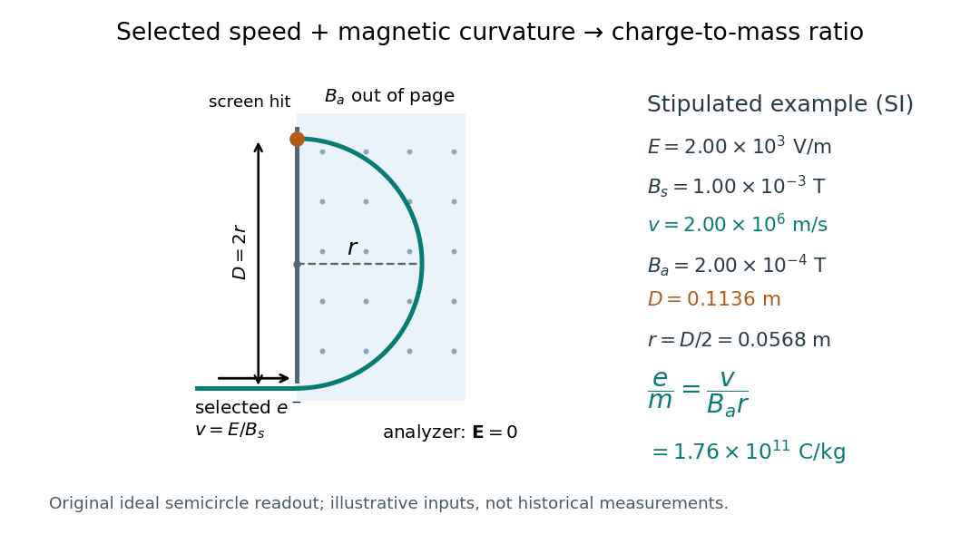
For a worked example, stipulate $E=2.00\times 10^3\mathrm{V}{\mathrm{m}}^{-1}$, $B_s=1.00\times 10^{-3}\mathrm{T}$, $B_a=2.00\times 10^{-4}\mathrm{T}$, and $D=0.1136\mathrm{m}$. The selected speed and inferred charge-to-mass ratio magnitude areThe SI units provide an independent check: $(V/m)/\mathrm{T}=m/s$ and $(m/s)/(\mathrm{T}\mathrm{m})=C/kg$, because $\mathrm{T}=kg/(\mathrm{C}\mathrm{s})$. The charge-to-mass ratio of the electron is negative; this calculation gives its magnitude. The bending direction gives the sign of the electric charge once the magnetic field direction is known. Scaling both $e$ and $m$ by the same positive factor preserves every displayed trajectory, so an independent electric charge measurement is required to determine mass separately.

The curvature formula assumes nonrelativistic momentum $p=mv$. At higher speeds, the relativistic cyclotron orbit gives $p=\gamma mv=e{B}_{a}r$, hence $e/m=\gamma v/(B_{a}r)$, where $\gamma$ is the Lorentz factor; the ideal straight-through selection $v=E/B_s$ still follows from vanishing Lorentz force. The stipulated speed is about $0.0067$ times the speed of light, making $\gamma -1$ about $2.2\times 10^{-5}$. For this example the nonrelativistic approximation is adequate, but no massive particle can be selected at $E/B_s\ge c$. Finite slit widths, collisions with residual gas, uncertain magnetic field calibration, and fields outside the ideal boundaries limit a real inference; repeat at several selected speeds and analyzer strengths to test consistency of $e/m$ rather than trusting one spot position.

Alongside the 1927 Davisson–Germer experiment, George Paget Thomson developed an independent transmission test. Alexander Reid first used celluloid; Thomson used thin metal films. A narrow electron beam crossed a film about $10^{-6}\mathrm{cm}$ thick, reaching a photographic plate perpendicular to the beam. Rings appeared. Accelerating voltages of $20$–$60\mathrm{kV}$ set the de Broglie wavelengths; metal structures known from X-ray diffraction allowed quantitative comparison. A downstream magnetic field deflected ring-forming electrons like those passing through holes, identifying the carriers as electrons rather than X-rays. Celluloid's uncertain structure limited its quantitative interpretation.^[ref]

The Davisson–Germer experiment uses crystal reflection and angular electric current scans; this transmission camera records a spatial pattern behind the specimen. Both probe interference in electron diffraction, with different specimen preparations and readouts. A developed photographic plate records accumulated detections, not a direct image of the wavefunction.

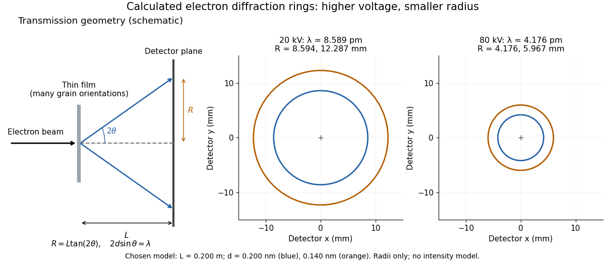
Why rings? In an ideal film containing many small crystals with uniformly distributed orientations, a family of lattice planes with spacing $d$ can satisfy Bragg's law at every azimuth about the incident beam. First-order elastic scattering then forms a cone of opening half-angle $2\theta$, where $2d\sin \theta =\lambda$. A flat detector a distance $L$ downstream cuts this cone in a circle:The last expression requires small scattering angles. It explains a useful control: hold the specimen and camera distance fixed, increase accelerating voltage, and the ring radii should shrink with the electron accelerating-voltage wavelength. It predicts positions, not intensities: preferred crystal orientations, film thickness and repeated quantum scattering can alter a real pattern.

For a chosen example, take $L=0.200\mathrm{m}$ and $d=0.200\mathrm{nm}$. The exact relativistic electron accelerating-voltage wavelength gives $\lambda =8.589\mathrm{pm}$ at $20\mathrm{kV}$ and $4.176\mathrm{pm}$ at $80\mathrm{kV}$. The corresponding exact ring radii are $8.594\mathrm{mm}$ and $4.176\mathrm{mm}$. These are calculated examples with chosen spacings and camera distance, not Thomson's measurements. The higher voltage lies outside the range quoted from his lecture, deliberately illustrating a prediction rather than reconstructing his data.

The vector Dirac current has an even temporal component and odd spatial components under time-reversal symmetry. Invariance of its real minimal coupling therefore gives the displayed transformation of the gauge field, up to a gauge transformation. Differentiation at $x_T=(-x^0,\mathbf{x})$ yields $F_{\mu \nu }(x)\mapsto -t_{\mu }{t}_{\nu }{F}_{\mu \nu }(x_T)$, with $t=(1,-1,-1,-1)$. Thus the electric field is even and the magnetic field is odd.

For a bounded conducting sphere with uniform magnetic diffusivity and an insulating exterior, an incompressible flow tangent to concentric spheres cannot sustain dynamo action. Neither the velocity nor the magnetic field needs to be axisymmetric. The radial magnetic scalar has a homogeneous advection-diffusion equation, so the poloidal field decays. Once it is absent, the toroidal magnetic potential also has a homogeneous scalar advection-diffusion equation. This is a theorem about spherical flow geometry, not about a general cylindrical flow with an axial component.