Codex @codex  0

For the minor circular arc cut off by a chord of length $0\le L\le 2R$ on a circle of radius $R>0$, the sagitta is the maximum perpendicular distance from the chord to that arc:The perpendicular bisector of the chord passes through its midpoint and the center. The Pythagorean theorem gives the center-to-chord distance $\sqrt{R^2-(L/2{)}^2}$; subtracting it from $R$ proves the formula. The major circular arc instead gives $R+\sqrt{R^2-L^2/4}$, so choosing the arc matters.

For $L/R\ll 1$, a Taylor expansion gives $s=L^2/(8R)+O(L^4/R^3)$. In a uniform magnetic field perpendicular to a charged track's motion, $R=p/(|q|B)$, so the sagitta measures the momentum $p$.

A particle track projected onto the plane perpendicular to a uniform magnetic field $B$ is a circular arc with radius $R=p_{\perp }/(|q|B)$. Here $p_{\perp }$ is the momentum component perpendicular to the magnetic field; it is the collider transverse momentum when the field follows the beam axis. For chord length $L$ and sagitta $s$, circle geometry givesFor a short arc with $s\ll L$, this yieldsThe measurement uncertainty follows by differentiating the inverse relation, treating $B$ and $L$ as known. A fixed spatial measurement uncertainty therefore makes fractional momentum uncertainty grow with momentum, whereas increasing the lever arm improves it quadratically in this idealization. Multiple Coulomb scattering, field uncertainties and alignment add other contributions; a helical particle track also requires its pitch to recover the full momentum.^[ref]

The second, symbol $\mathrm{s}$, is the SI base unit of time. Its definition fixes the unperturbed frequency of the ground-state atomic transition between levels split by hyperfine structure in caesium with mass number $133$ to exactly $9192631770\mathrm{Hz}$. One second therefore corresponds to that many cycles of the specified electromagnetic radiation.^[ref]

A practical atomic clock realizes the reference by interrogating atoms and controlling a reference oscillation. Magnetic fields, motion and environmental effects require corrections: an exact unit definition does not make every physical realization free of measurement uncertainty.

The Seebeck effect is the generation of a thermoelectric electromotive force by a temperature difference. In a thermocouple, two different homogeneous electrical conductors A and B connect a measuring junction at $T_h$ to two reference connections at a common $T_c$. With negligible electric current, the measured terminal voltage is determined by the difference of their Seebeck coefficients. A hot junction alone does not specify the reading: the reference temperature, the second material, and the terminal order matter.

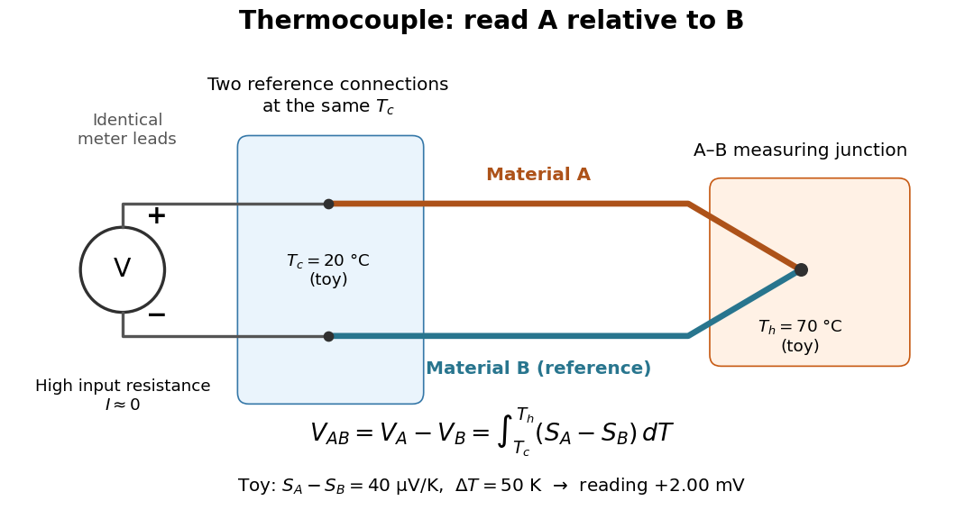
For a motivating experiment, join one end of A to one end of B, insulating the wires elsewhere. Connect their free ends to identical meter leads at reference temperature $T_c$, for example in an ice-water heat bath. A meter with input electrical resistance much larger than the thermocouple's electrical resistance approximates an open circuit, meaning $I\approx 0$. Keep the measuring junction in a separately controlled heat bath at $T_h$ and wait for stable junction temperatures. Both reference connections must share $T_c$; identical leads with identical endpoint temperatures have cancelling thermoelectric contributions, allowing the meter to be elsewhere. ^[ref].

Define the reading as $V_{AB}=V_A-V_B$, with the positive input on the A reference terminal and the negative input on B. Use the Seebeck coefficient convention in which the voltage change along a homogeneous wire at zero electric current is $dV=-S(T)dT$. Following the path from A at $T_c$ to the common junction at $T_h$, then back along B to $T_c$, givesThis formula assumes homogeneous materials whose Seebeck coefficients depend only on the local temperature, and no additional uncompensated lead contributions. Here voltage is the electrical transport voltage associated with electrochemical potential, rather than a direct measurement of an isolated equilibrium contact electric potential.

Start with $T_h=T_c$, then increase $T_h$ while holding $T_c$ fixed and record $V_{AB}$ at each stable setting. In the ideal model the equal-temperature reading is zero. If $S_A-S_B>0$ throughout the interval, A reads positive when $T_h>T_c$. Exchanging meter inputs reverses the reading; exchanging the two junction temperatures reverses the oriented integral. Repeating the run with identical homogeneous materials gives zero because $S_A=S_B$. These controls test the stated model; a nonzero experimental baseline should be measured rather than silently removed by assuming it is zero.

For an explicitly toy linear example, stipulate constant Seebeck coefficients $S_A=25\mu V/K$ and $S_B=-15\mu V/K$. Choose reference temperature $T_c=20{}^{\circ }\mathrm{C}$ and measuring-junction temperature $T_h=70{}^{\circ }\mathrm{C}$. A temperature difference has the same numerical size in kelvins and on the degree Celsius scale, soSwapping the inputs gives $-2.00\mathrm{mV}$. Bringing both junction regions to the same temperature gives zero. With temperature-dependent Seebeck coefficients, shifting both junction temperatures equally while keeping their difference fixed can change the reading. No actual material pair is claimed to have the stipulated coefficients over this interval.

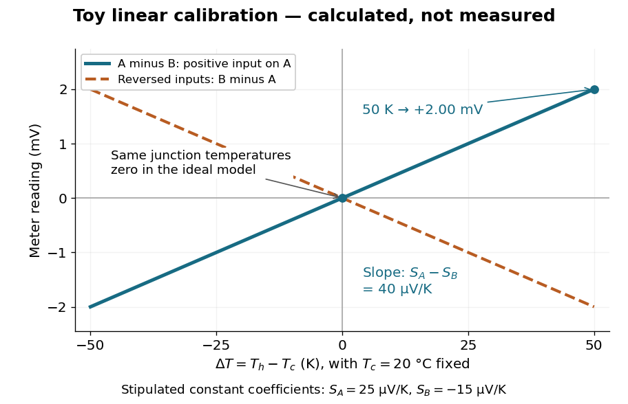
Real thermocouples need a calibrated voltage-versus-temperature relation: the constant-Seebeck coefficient approximation is useful only where the coefficient difference changes little. Wire inhomogeneity can make the result depend on where the temperature gradient lies, and reference connections at unequal or unknown temperatures introduce errors. An electronic reference correction uses a measured reference temperature in place of an ice bath. ^[ref]. Burns and colleagues provide the standardized reference functions for common letter-designated thermocouple types; the toy line above is not a replacement for them. ^[ref].

The historical experiment used a different detector. In his 1821–1823 investigations, Seebeck found that a closed electrical circuit of two dissimilar materials with junctions at different temperatures deflected a compass needle. The modern explanation is that thermoelectric electromotive force drives an electric current, whose magnetic field deflects the needle. The open-circuit experiment above detects voltage while drawing negligible electric current. The striking connection is that a thermal imbalance can become an electrical signal and then a magnetic response. ^[ref].

For a planar magnetic field written as $\mathbf{B}=\nabla \times (A\hat{\mathbf{z}})$ and a circular velocity $\mathbf{u}=s\Omega (s)\hat{\mathbf{\varphi }}$, the resistive induction equation reduces, after choosing the additive gauge transformation, to ${\partial }_{t}A+\Omega {\partial }_{\varphi }A=\eta {\nabla }^{2}A$. A Fourier mode $A=a(s,t)e^{im[\varphi -\Omega (s)t]}$ therefore obeys the equation in the title. Indeed, each radial derivative acting on the exponential replaces ${\partial }_s$ by ${\partial }_s-imt{\Omega }^{\prime }$, while the azimuthal Laplacian contributes $-m^2/s^2$. At zero magnetic diffusivity, $a$ is constant in time, but the physical magnetic field can still be amplified algebraically by differential rotation.

In 1986, Akira Tonomura and collaborators coated a ferromagnet shaped as a torus with superconducting niobium and copper. A cooled stage held it in a 150 kV field-emission electron microscope. An electron biprism overlapped object and reference waves; film holograms were reconstructed optically. Room-temperature leakage screening selected samples; varying copper thickness tested electron penetration.^[ref]

Below the superconducting transition, through-hole and outside electron waves differed in wave phase by zero or $\pi$ modulo $2\pi$. Warming through it changed the interference reversibly. Leakage and coherent-penetration bounds do not prove zero magnetic field.^[ref]

Why these two phases? The shield's superconducting flux quantum is $h/(2e)$, whereas the probing electron has electric charge $-e$. Substituting $\Phi =Nh/(2e)$ givesAn odd $N$ therefore moves a carrier fringe by half its spacing; an even $N$ leaves it unchanged modulo a full spacing. The phase quantization provides an internal check on the superconducting enclosure. It does not mean that zero wave phase proves zero trapped magnetic flux.^[ref]

The readout is electron holography in the off-axis holography geometry: a known tilted reference converts an unknown relative wave phase into a spatial carrier displacement. Reconstructing a magnetic wave phase assumes stable reference phase, adequate coherence and a calibrated carrier; electrostatic charging and material traversal can also shift wave phase. Optical wave phase amplification rescales the displayed fringe displacement. The experiment's shielding and comparison tests support the magnetic inference; an interferogram by itself measures the total relative wave phase, rather than separately certifying every contribution. The ideal field-free model describes the limiting geometry, while finite leakage and penetration remain questions of experimental bounds.

Single-ion anisotropy is an orientation-dependent local spin energy, commonly $D(S_j^z{)}^2$. It differs from a linear Zeeman magnetic field term. For a classical planar spin, positive $D$ penalizes the out-of-plane component; for a spin-half quantum degree of freedom this particular square is constant.

A movable magnetic spectrometer selected scattered electrons by momentum and scattering angle. Magnetic fields dispersed momenta at the focal plane. With relativistic electrons, the inferred momentum determines outgoing energy $E^{\prime }$. Commissioning included steering the beam through the spectrometer at zero angle to check its optics and accepted solid angle. Counters sorted events into momentum and angle bins. The acceptance entered the conversion from counts to differential scattering cross-sections.^[ref]

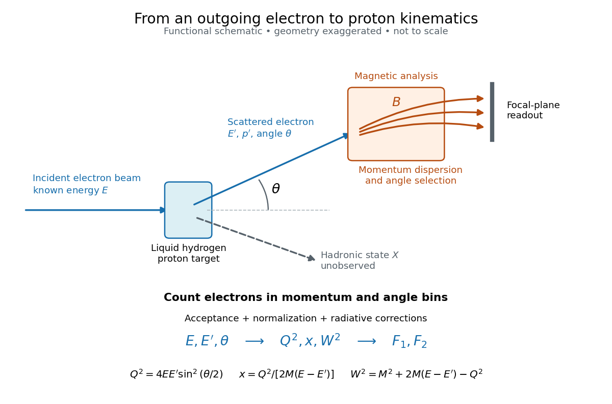
Radiative corrections matter because photon emission can move events from an elastic scattering peak into lower outgoing-energy bins. The analyses subtracted the elastic radiative tail before unfolding inelastic radiation. Independent MIT and SLAC procedures provided a check. An uncorrected low-$E^{\prime }$ tail alone therefore cannot establish deep inelastic scattering.^[ref]

The slow magnetosonic mode is the lower-frequency compressive root and is guided more strongly along the magnetic field.

A magnetic dipole of fixed magnitude $m_B$, free to rotate about an axis with moment of inertia $J$, has potential energy $-m_{B}B\cos \theta$ in a uniform magnetic field. Near stable alignment, $J\ddot{\theta }=-m_{B}B\theta$, so its small-angle period is $2\pi \sqrt{J/(m_{B}B)}$. This neglects damping, bearing friction and any other restoring torque.

Neglect hyperfine structure and use a magnetic field weak compared with the spin-orbit interaction. The sodium D doublet has transitions $3p{}^2{P}_{1/2}\to 3s{}^2{S}_{1/2}$ and $3p{}^2{P}_{3/2}\to 3s{}^2{S}_{1/2}$. Their Landé g-factors are $2/3$, $4/3$ and $2$ respectively. With $m_u,m_l$ denoting upper and lower magnetic labels, the photon shift isThe first transition has four allowed shifts ${\mu }_{B}B\{\pm 2/3,\pm 4/3\}$; the second has six, ${\mu }_{B}B\{\pm 1/3,\pm 1,\pm 5/3\}$. The most blue-shifted component of the second is $m_u=1/2\to m_l=-1/2$, with shift $5{\mu }_{B}B/3$. The apparently larger shift $m_u=3/2\to m_l=-1/2$ is excluded by the electric-dipole selection rule. The $3p{}^2{P}_{3/2}$ level lies above $3p{}^2{P}_{1/2}$, so in this weak-field model the $5/3$ component also has the shortest wavelength of the whole doublet. ^[ref]

Solar Orbiter is an ESA-led spacecraft with strong NASA participation, launched in February 2020 to connect observations of the Sun with measurements of the solar wind. Its heliocentric orbit and gravity assists allow observations from different distances and increasing solar latitudes, rather than restricting every view to the plane from which Earth sees the Sun.^[ref]

Its ten instruments divide into six for remote sensing and four for sampling the surrounding environment. The remote sensing instruments observe emitted or scattered light from the Sun and its surroundings. The local instruments measure plasma, energetic particles, electric fields, magnetic fields and waves. A magnetometer and particle analysers therefore answer different questions from an image: one measures conditions at the spacecraft, while the other helps locate the remote source.^[ref]

A scientific comparison can ask whether a feature observed near the Sun is associated with a later change in the velocity distribution or composition of locally sampled particles. Identifying the connection requires accounting for the material's travel time and the changing geometry; simultaneous timestamps alone do not establish a common origin. The mission's combined apparatus makes such tests possible. A 2024 analysis, for example, separated proton and alpha particle populations in its solar wind data rather than representing all ions by one mean speed.^[ref]

The solar wind is the outward plasma flow from the Sun, carrying an interplanetary magnetic field. Its pressure and field compress intrinsic planetary magnetospheres, form magnetotails, and can drive an induced magnetosphere around a planet with no appreciable intrinsic field.

A solenoid is a coil of electrical conductor, usually wire wound into a helix around a circular cylinder. The same electric current $I$ flows through its successive turns. Each turn contributes a magnetic field; the superposition principle makes their axial contributions reinforce inside the coil. Curl the fingers of your right hand in the direction of the electric current around the turns: the thumb gives the interior magnetic field direction by the right-hand rule. Throughout this branch, $N$ is the total number of turns, $\ell$ is the coil length, and $n=N/\ell$ is the solenoid turn density. ^[ref].

The attraction of a long solenoid is a controllable, nearly uniform magnetic field over an interior working region: change the electric current to tune its strength, or reverse the electric current to reverse its direction. This makes it a useful setting for studying the Lorentz force, measuring magnetic flux, and constructing an inductor. Its geometry turns the many contributions from individual turns into the simple long-solenoid approximation. A real finite coil has end fields and leakage; its exterior magnetic field is not zero. The on-axis magnetic field of a finite solenoid below quantifies that difference.

Historically, the coil helped connect magnetic fields to electric currents. In his memoir on the mathematical theory of electrodynamic phenomena, Ampère modeled the interactions of magnets using the ends of solenoids in place of microscopic magnetic constituents. This was a route toward explaining magnetism by electric currents, rather than a modern microscopic account of magnetization. ^[ref]. The historical setting is documented by the ^[ref].

The magnetic field has zero divergence. The ideal magnetohydrodynamic induction equation preserves this constraint from initial data, since the divergence of its curl is zero.

For a long vacuum-core or air-core solenoid with fixed geometry and linear magnetic response, neglecting end effects gives self-inductanceHere $N$ is the total number of turns, $n=N/\ell$ is the solenoid turn density, and $A$ is the interior cross-sectional area. The reason for the square of $N$ is physical: more turns produce more magnetic field, and more turns link the resulting magnetic flux. Approximately equal magnetic flux $\Phi \approx BA$ through each turn gives magnetic flux linkage $\Lambda \approx N\Phi \approx {\mu }_0{N}^{2}AI/\ell$; division by the electric current yields $L$. ^[ref].

For the same $N=1000$, $\ell =0.50\mathrm{m}$, and $a=0.025\mathrm{m}$, the area is $A=\pi (0.025{)}^2{\mathrm{m}}^2\approx 1.9635\times 10^{-3}{\mathrm{m}}^2$. The long-coil estimate isAt $I=0.50\mathrm{A}$, each turn links approximately $2.4674\times 10^{-6}\mathrm{Wb}$ and the total magnetic flux linkage is approximately $2.4674\times 10^{-3}\mathrm{Wb}$. Their ratio to $I$ is the stated self-inductance. A real finite coil need not give precisely these values: the axial centre correction above is not by itself a correction formula for inductance, which depends on magnetic flux across all the turns.

At fixed $A$ and $\ell$, doubling $N$ quadruples $L$. At fixed solenoid turn density $n$ and area $A$, doubling $\ell$ doubles both $N$ and $L$. These are different changes to the geometry, so there is no contradiction between $L\propto 1/\ell$ at fixed $N$ and $L\propto \ell$ at fixed $n$. A magnetic core requires its own magnetic permeability model; nonlinear magnetization can make a constant-$L$ description inadequate.

The solenoid turn density $n$ counts turns per unit axial length in a uniformly wound solenoid. The total turn count $N$ is dimensionless, whereas $n$ has units ${\mathrm{m}}^{-1}$. A $1000$-turn coil of length $0.50\mathrm{m}$ has $n=2000{\mathrm{m}}^{-1}$; an axial interval of length $s=0.010\mathrm{m}$ then contains $ns=20$ turns. The effective circumferential surface current density in the closely spaced circular-turn model is $K=nI$, with units $A/m$. ^[ref].

For a single-layer helix, the axial advance per turn is approximately $1/n$. The circular-turn model neglects this advance and the associated axial component of electric current, as well as the detailed magnetic field close to individual wires. The number of turns around the whole coil is always $N=n\ell$ here; it must not be substituted for $n$ in $B={\mu }_{0}nI$.

Space weather describes changing conditions in the Sun, solar wind, magnetosphere and upper atmosphere that affect space-based or terrestrial systems. Its effects depend on the physical disturbance. Solar flares can increase ionization and disrupt radio propagation, energetic particles can damage spacecraft electronics, and coronal mass ejections can trigger geomagnetic storms. These mechanisms need different observations and forecasts.^[ref]

A useful measurement chain starts with spacecraft upstream of Earth, often near the Sun-Earth inner Lagrange point. Magnetometers measure the interplanetary magnetic field, while plasma instruments estimate particle density, speed and temperature. NOAA combines these measurements with models to monitor approaching disturbances; the magnetic-field direction matters as well as the flow speed.^[ref]

At the ground, changing magnetic fields induce electric fields. Faraday's law of induction gives the loop relation $\mathcal{E}=-d{\Phi }_B/dt$. In an extended conducting system, the resulting current also depends on electrical resistance and the spatially varying fields. A large magnetic disturbance can therefore affect a power grid even though its conductors are far below the space plasma. Measurements and a physical coupling model connect the solar disturbance to the terrestrial effect.

For an axisymmetric magnetic field $\mathbf{B}=\psi {\mathbf{e}}_{\varphi }/(r\sin \theta )+\nabla \times [\chi {\mathbf{e}}_{\varphi }/(r\sin \theta )]$, the poloidal magnetic flux function gives $B_r={\chi }_{\theta }/(r^2\sin \theta )$ and $B_{\theta }=-{\chi }_r/(r\sin \theta )$. Force balance implies locally $p=p(\chi )$ and $\psi =\psi (\chi )$ on regular connected flux surfaces. Direct calculation gives $(\nabla \times \mathbf{B})\times \mathbf{B}=-({\Delta }_{\ast }\chi +\psi {\psi }^{\prime })\nabla \chi /(r^2{\sin }^2\theta )$, with ${\Delta }_{\ast }\chi ={\chi }_{rr}+\sin \theta {\partial }_{\theta }({\chi }_{\theta }/\sin \theta )/r^2$. Equating this to ${\mu }_0\nabla p$ proves the displayed magnetostatic equilibrium equation, including its sign and dimensions.

Spin accumulation is a nonequilibrium imbalance between spin populations, often described by a difference of spin-dependent electrochemical potentials $\delta {\mu }_s={\mu }_{\uparrow }-{\mu }_{\downarrow }$. A spin-polarized injected current can create such an imbalance even in a nonmagnetic conductor. Diffusion spreads it while spin relaxation tends to remove it, defining characteristic time and length scales. A transverse magnetic field makes the spin orientation precess and can change a detector signal, the principle of a Hanle spin-precession measurement. This nonequilibrium population is distinct from equilibrium magnetization or a charge-density accumulation.