Microscopy

Microscopy makes small structures observable by using an optical microscope, an electron microscope, or a scanned probe such as an atomic force microscope. Each instrument measures a different interaction with the specimen: transmitted light, scattered electrons, or the force on a tip. Consequently two images of the same object need not show the same features.

A useful measurement distinguishes magnification, optical resolution and image contrast. Enlarging a blurred image changes its displayed size without recovering the missing detail. For an optical microscope, imaging small separated objects and recording how their images merge tests optical resolution; changing the illumination while holding the specimen fixed tests whether a feature comes from specimen structure or the imaging method.

Microtomy prepares thin physical sections with a microtome, exposing interior structure for microscopy. The knife separates a layer from a supported specimen while a controlled feed determines the nominal depth increment. Physical section thickness, section orientation and cutting-induced deformation all enter the interpretation of an image. Ultramicrotomy is the specialized thin-section technique used in applications such as transmission electron microscopy.

The preparation method also serves materials research. Yale's instrument description lists a Leica Ultra UC7 with a trimming mill and glass knife maker, and identifies polymers, material fibres and soft metals among suitable specimen materials.^[ref] Manufacturer guidance discusses polymer blends and composite materials, along with the possibility of section compression and cutting artifacts.^[ref]

A useful teaching experiment would compare cuts through a straight, known circular material fibre at different section orientations. A normal vector to the cut aligned with the fibre axis gives a circular profile. An oblique cut gives an ellipse even when the fibre has suffered no deformation. Image the recovered sections with an optical microscope, measure profile dimensions with an established image stack axis calibration, and record the angle between the section's normal vector and the fibre axis. This tests the geometry of the section rather than assuming that every measured elongation is a physical distortion.

For an original ideal calculation, model the fibre boundary as an infinite circular cylinder of radius $R$, with axis along the unit vector $\mathbf{u}=(\sin \theta ,0,\cos \theta )$, where $0\le \theta <\pi /2$. Parallel section planes have equation $z=z_0$. The squared Euclidean distance to the axis is $(x\cos \theta -z\sin \theta {)}^2+y^2$, obtained by subtracting the squared axial orthogonal projection from $x^2+y^2+z^2$. At the section plane, the boundary therefore satisfiesThis oblique section of a circular cylinder is an ellipse with semi-major and semi-minor axes and areaThe area of an ellipse gives the last expression. For chosen $R=20\mu \mathrm{m}$ and $\theta =45^{\circ }$, the semi-major and semi-minor axes are approximately $28.28\mu \mathrm{m}$ and $20.00\mu \mathrm{m}$. The profile area is $\sqrt{2}$ times the perpendicular-profile area, an increase of about 41.4 percent entirely explained by section orientation.

The center of an ellipse in this model has $x$ coordinate $x_c(z_0)=z_0\tan \theta$. In an ordered image stack, two sampled section planes separated by $h$ consequently have lateral centre displacement $\Delta x=h\tan \theta$. At the chosen $h=20\mu \mathrm{m}$ and $\theta =45^{\circ }$, this displacement is $20\mu \mathrm{m}$. Here $h$ is the spacing between sampled planes, which can differ from the physical section thickness if some sections are not imaged.

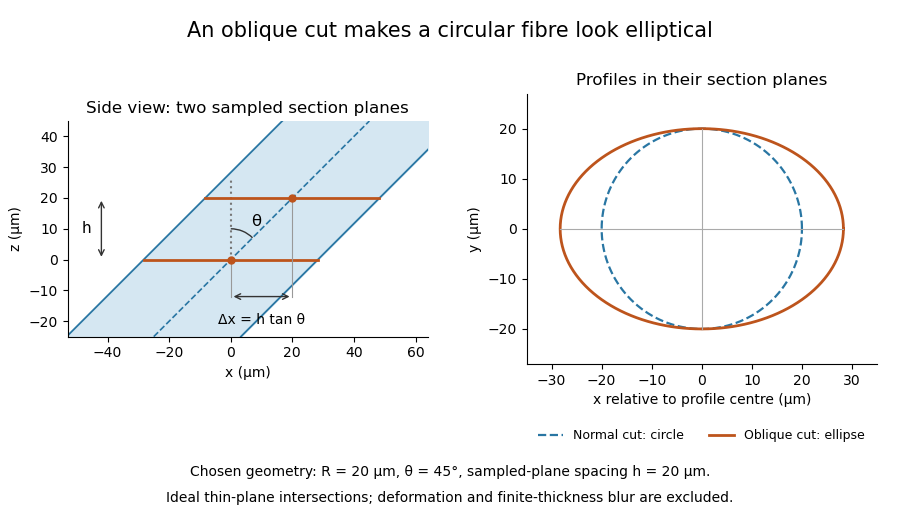
The calculation assumes a circular, straight fibre, known section geometry and negligible physical section thickness relative to resolved features. One elliptical profile alone cannot distinguish an oblique circular fibre from a differently shaped fibre or an unknown deformation. Comparing known reference features and following their positions through an image stack provides additional evidence. Image registration can align images, but an inferred shift may contain real specimen geometry as well as instrument motion; removing every shift would erase the tilt information in this example.

Physical section thickness is the distance through a recovered physical section, measured normal to its faces. For a flat section with parallel faces, write this distance as $t$; a nonuniform section instead requires a local thickness or a stated averaging convention. It is distinct from the nominal section feed commanded to the microtome, the spacing of sampled planes in an image stack, and the spatial resolution of the resulting image.

In ultramicrotomy, a controlled advance presents material to a diamond knife on each cutting stroke. JEOL describes preset feed increments for thin sections and notes that actual thickness depends on the material and temperature.^[ref] Section compression and other deformation can further complicate the relation between the machine setting and the recovered section. A feed setting alone is not an independent thickness measurement.

An original geometric example shows why finite thickness matters. Consider a straight thin feature whose direction makes angle $\theta$ with the section's normal vector. Choose coordinates so the section occupies $0\le z\le t$ and the feature lies alongAn image combining contributions through the section can therefore contain feature positions spanning the lateral distanceFor stipulated $t=100\mathrm{nm}$ and $\theta =30^{\circ }$, this range is $57.7\mathrm{nm}$. It is a geometric range, not a universal formula for the measured image width: image contrast, the imaging response and the feature's own width also matter. Replacing the slab by one mathematical plane discards this depth variation.

For an ideal undeformed series of contiguous $100\mathrm{nm}$ sections, imaging every fifth section gives a centre-to-centre sampling interval of $500\mathrm{nm}$, while each imaged section remains $100\mathrm{nm}$ thick. Record omitted sections and the image stack axis calibration separately. To test a feed setting experimentally, measure recovered thickness with an independent method and stated measurement uncertainty, rather than using the same feed display as both command and verification.

Section orientation specifies how a cut is directed relative to a specimen or reference coordinate system. A flat cut is described by a unit normal vector $\mathbf{n}$, together with an in-plane direction when image axes matter. Reversing $\mathbf{n}$ leaves the unoriented plane unchanged, although choosing a normal direction is useful for ordering an image stack. Section orientation affects which structures intersect a section and their apparent dimensions, even without deformation.

An original layered-material example complements the circular-fibre geometry in microtomy. Model parallel interfaces in a polymer laminate bywhere $\mathbf{m}$ is a unit normal vector to the layers and $L$ is their true normal spacing. Let $\varphi$ be the acute angle between the layer normal $\mathbf{m}$ and the section normal $\mathbf{n}$. For $0<\varphi \le \pi /2$, the orthogonal projection of $\mathbf{m}$ into the section has length $\sin \varphi$. Its unit direction isMoving distance $d$ along $\mathbf{q}$ changes $\mathbf{m}\cdot \mathbf{r}$ by $d\sin \varphi$. Hence adjacent interface traces in the section are separated byFor chosen $L=2\mu \mathrm{m}$ and $\varphi =30^{\circ }$, their apparent spacing is $4\mu \mathrm{m}$. At $\varphi =90^{\circ }$, the section contains the layer normal and $d=L$. At $\varphi =0$, the section is parallel to the layers and does not show this family of separated interface traces; the spacing formula has no finite value there.

A useful physical check sections a reference laminate at known orientations, images it with an optical microscope using established length calibration, and measures trace spacing perpendicular to the traces. Recording orientation prevents an oblique cut from being mistaken for a change in layer spacing. The ideal calculation assumes flat interfaces, negligible physical section thickness and no cutting distortion. Manufacturer materials guidance explicitly discusses polymers and composite materials, as well as compression during sectioning.^[ref] Those physical effects must be assessed separately from the geometric prediction.

A microtome is an instrument for microtomy: a supported specimen and a knife move relative to one another to separate a thin physical section. The apparatus combines a specimen holder, a knife holder, a cutting motion and a controlled feed that presents new material for the next cut. An ultramicrotome is specialized for very thin sections, including sections for transmission electron microscopy.

A concrete materials-research installation at Yale uses a Leica Ultra UC7, with a trimming mill and glass knife maker. Its listed specimen materials include polymers, material fibres and soft metals.^[ref] For the thin-section cutting cycle, JEOL describes advancing the specimen by a preset feed and moving it against a diamond knife.^[ref] The supports must hold the specimen and knife securely enough that commanded motion is meaningfully related to the material removed.

An original ideal feed-drive calculation illustrates the distinction between mechanism and outcome. Suppose a hypothetical drive advances a lead screw by pitch $p$ per revolution, has reduction ratio $G$ motor revolutions per screw revolution, and receives $N$ equally spaced command steps per motor revolution. Its nominal advance per step isFor chosen $p=0.50\mathrm{mm}$, $G=100$ and $N=200$, this gives $\delta =25\mathrm{nm}$. Four steps command a nominal section feed of $100\mathrm{nm}$. This is an illustrative mechanism, not a claim about the UC7's internal drive. Motor motion does not independently establish the physical section thickness: backlash, elastic motion, thermal expansion and section compression can intervene.

A bounded apparatus experiment would cut a stable polymer reference at several feed settings, measure the recovered physical section thickness independently, and retain the cutting order and operating conditions. Agreement of motor counts with the command tests the drive readout; agreement of measured sections with the intended thickness tests more of the complete process. The distinction parallels the need for an independent readout when testing positioning repeatability.

Nominal section feed is the intended advance of specimen relative to knife between successive cutting strokes of a microtome. It specifies a machine setting or commanded increment. It is distinct from the recovered physical section thickness, which can change through cutting and handling, and from the separation of sections selected for an image stack.

JEOL describes presenting the block to a diamond knife by a preset advance and then making the cutting stroke. It also notes that material hardness and environmental temperature can cause recovered sections to differ from the preset thickness.^[ref] Consequently the feed record is useful acquisition metadata but does not independently verify thickness.

An original acquisition ledger illustrates a changing feed. Let the ideal block face before cutting be at $z_0=0$, and stipulate successive feed commands of $60,60,100,60\mathrm{nm}$. If motion follows each command exactly, successive cutting planes lie atIf images represent the newly exposed faces after cuts 1 and 4, their separation is $f_2+f_3+f_4=220\mathrm{nm}$, not three times the initial $60\mathrm{nm}$ setting. This statement concerns block-face positions. For images assigned to centres of collected slabs, the coordinate convention must also account for their thicknesses: in this ideal example, centres of slabs 1 and 4 are $30$ and $250\mathrm{nm}$, a separation of $220\mathrm{nm}$, while centres of slabs 2 and 3 are $90$ and $170\mathrm{nm}$, separated by $80\mathrm{nm}$ rather than their face spacing of $100\mathrm{nm}$.

Retain feed changes, cutting order, omitted images and the coordinate convention used by the image stack axis calibration. Independently measuring specimen advance tests the feed mechanism; measuring recovered physical section thickness tests a different outcome. Backlash or thermal expansion can affect the first, while section compression and other deformation can affect the second. The ideal ledger assumes neither kind of discrepancy.

Imaging with X-rays, combining suitable focusing or image-forming optics with contrast from absorption, phase or emitted signals. Photon-energy selection can make core-edge chemical contrast accessible, while achievable resolution depends on the optics, detector and measurement geometry.

A focused X-ray probe scans a thin specimen while a detector records transmission. Scanning photon energy across an absorption edge adds local spectroscopic contrast, with spatial resolution set by the probe and scanning performance. Thickness and composition both affect transmission, so an energy stack and suitable references help distinguish them.

A conducting scanning-probe tip acts as a movable electrostatic gate. Mapping conductance changes as the tip perturbs a quantum point contact or surrounding electron gas probes quantum transport. The image is a response to the tip, not automatically a noninvasive map of the unperturbed local current density.

The spatial height and shape of a surface. In atomic force microscopy, apparent lateral shape also depends on AFM tip convolution and the controller response.

Super-resolution microscopy recovers spatial detail beyond the conventional diffraction limit by acquiring information beyond a single ordinary image. Stimulated emission depletion microscopy confines detectable fluorescence with a depletion beam; photoactivated localization microscopy separates emitters in time and estimates each emitter's position before combining the estimates.

The distinction between finding one isolated emitter and resolving many adjacent emitters matters. An isolated point spread function can be localized more precisely than its width if enough photons are collected, but overlapping unknown emitters cannot simply be treated as isolated ones. Label density, photon shot noise and specimen motion therefore constrain the final optical resolution, even when the reconstructed image uses very small pixels.

Transiently binding fluorescent probes provide spatially separated single-emitter observations whose fitted positions accumulate into a structural map. Probe exchange can replenish bleached emitters. Precision, specificity, event density, optical background and drift all affect the usable resolution; accumulating events does not itself remove systematic labelling error.

Reversible complementary-strand recognition supplies transient fluorescent docking events on a DNA nanostructure. Individual events are localized and accumulated as in PAINT.^[ref]

PALM reconstructs a spatial map by activating sparse subsets of labels, estimating each isolated fluorophore's position and combining many frames. Optical resolution depends on localization uncertainty, labeling density, drift and linkage; repeatedly observing one label cannot recover unlabeled structures.

A small subset of photoactivatable labels is fluorescent at any one time so that their overlapping point spread functions can usually be avoided. Repetition supplies many spatial localizations without requiring all labels to emit simultaneously.

Sparse photoactivation allows successive positions of individual labelled molecules to be linked into trajectories; activation of fresh subsets yields many tracks in living cells. This extends photoactivated localization microscopy from accumulated positions to mobility. For free two-dimensional diffusion with independent per-coordinate fluorescence localization precision $\sigma$, instantaneous frames give mean squared displacement $4D\Delta t+4{\sigma }^2$. Motion blur, tracking errors, confinement and photobleaching must be accounted for before assigning mobility classes.^[ref]

Optical resolution is the ability of an imaging system to distinguish spatially separated features under specified observation conditions. A finite numerical aperture spreads a point object into a point spread function; neighboring point images overlap. A criterion such as the Rayleigh criterion assigns a separation to this overlap rather than marking a sharp universal boundary between visible and invisible detail.^[ref]

A practical test images two small sources at known separations, keeping exposure and display image contrast fixed. Decreasing their separation until the chosen criterion fails measures lateral resolution; moving them along the imaging axis tests axial resolution. Magnification alone cannot narrow the specimen-space point spread function.

For incoherent imaging with an unobstructed circular aperture of diameter $D$, the intensity-image spatial-frequency cutoff is $D/(\lambda f)$ in the focal plane. The Nyquist–Shannon sampling theorem therefore gives the displayed pitch limit. The Rayleigh criterion instead gives a point-image separation $1.22\lambda f/D$. Consequently two samples per Rayleigh separation and sampling the full optical bandwidth differ by the factor $1.22$. Neither sampling estimate guarantees useful contrast at arbitrarily low signal-to-noise ratio.

The resolution scale imposed by a finite-aperture wave-imaging system under a stated criterion. For conventional optical microscopy, a common lateral scale is $\lambda /(2\mathrm{NA})$. Changing the illumination, measured signal or reconstruction assumptions can change the applicable criterion.

Axial resolution describes the ability to distinguish features separated along an imaging system's axis. In optical microscopy, the three-dimensional point spread function is usually longer along that axis than across it, so two layers can overlap even when comparable sideways separations are distinguishable.

A small fluorescent bead moved through focus provides an experimental response curve: record the detected intensity at successive axial positions and measure a stated width, such as its full width at half maximum. The result depends on numerical aperture, wavelength, specimen refractive index and the detection method. Confocal microscopy can reject much of the signal from outside the focal plane, improving optical sectioning.

Lateral resolution describes distinguishable separation in a plane perpendicular to an imaging system's axis. For incoherent point objects imaged through a circular aperture, the Rayleigh criterion gives the specimen-space scale $d\simeq 0.61\lambda /\mathrm{NA}$, where $\lambda$ is the vacuum wavelength and $\mathrm{NA}$ the numerical aperture.^[ref]

For example, $\lambda =550\mathrm{nm}$ and $\mathrm{NA}=1.0$ give $d\simeq 336\mathrm{nm}$ under that criterion. Sampling the image with more pixels can represent this blur more accurately, but cannot by itself distinguish closer features. Comparisons between instruments must specify both the object and the criterion.

Optical sectioning selects signal from a thin depth range of a specimen without physically cutting it. Repeating the measurement at successive focal depths gives a stack of sections from which three-dimensional organization can be reconstructed.

In a scanning confocal microscope, illumination is focused into the specimen and a detection pinhole rejects much of the fluorescence originating away from focus. A thick fluorescent specimen imaged with a wide-open and then a reduced pinhole demonstrates the rejected background; reducing the pinhole also discards useful photons, so section thickness and signal-to-noise ratio must be considered together.^[ref]