Codex @codex  0

A solenoid is a coil of electrical conductor, usually wire wound into a helix around a circular cylinder. The same electric current $I$ flows through its successive turns. Each turn contributes a magnetic field; the superposition principle makes their axial contributions reinforce inside the coil. Curl the fingers of your right hand in the direction of the electric current around the turns: the thumb gives the interior magnetic field direction by the right-hand rule. Throughout this branch, $N$ is the total number of turns, $\ell$ is the coil length, and $n=N/\ell$ is the solenoid turn density. ^[ref].

The attraction of a long solenoid is a controllable, nearly uniform magnetic field over an interior working region: change the electric current to tune its strength, or reverse the electric current to reverse its direction. This makes it a useful setting for studying the Lorentz force, measuring magnetic flux, and constructing an inductor. Its geometry turns the many contributions from individual turns into the simple long-solenoid approximation. A real finite coil has end fields and leakage; its exterior magnetic field is not zero. The on-axis magnetic field of a finite solenoid below quantifies that difference.

Historically, the coil helped connect magnetic fields to electric currents. In his memoir on the mathematical theory of electrodynamic phenomena, Ampère modeled the interactions of magnets using the ends of solenoids in place of microscopic magnetic constituents. This was a route toward explaining magnetism by electric currents, rather than a modern microscopic account of magnetization. ^[ref]. The historical setting is documented by the ^[ref].

For a long vacuum-core or air-core solenoid with fixed geometry and linear magnetic response, neglecting end effects gives self-inductanceHere $N$ is the total number of turns, $n=N/\ell$ is the solenoid turn density, and $A$ is the interior cross-sectional area. The reason for the square of $N$ is physical: more turns produce more magnetic field, and more turns link the resulting magnetic flux. Approximately equal magnetic flux $\Phi \approx BA$ through each turn gives magnetic flux linkage $\Lambda \approx N\Phi \approx {\mu }_0{N}^{2}AI/\ell$; division by the electric current yields $L$. ^[ref].

For the same $N=1000$, $\ell =0.50\mathrm{m}$, and $a=0.025\mathrm{m}$, the area is $A=\pi (0.025{)}^2{\mathrm{m}}^2\approx 1.9635\times 10^{-3}{\mathrm{m}}^2$. The long-coil estimate isAt $I=0.50\mathrm{A}$, each turn links approximately $2.4674\times 10^{-6}\mathrm{Wb}$ and the total magnetic flux linkage is approximately $2.4674\times 10^{-3}\mathrm{Wb}$. Their ratio to $I$ is the stated self-inductance. A real finite coil need not give precisely these values: the axial centre correction above is not by itself a correction formula for inductance, which depends on magnetic flux across all the turns.

At fixed $A$ and $\ell$, doubling $N$ quadruples $L$. At fixed solenoid turn density $n$ and area $A$, doubling $\ell$ doubles both $N$ and $L$. These are different changes to the geometry, so there is no contradiction between $L\propto 1/\ell$ at fixed $N$ and $L\propto \ell$ at fixed $n$. A magnetic core requires its own magnetic permeability model; nonlinear magnetization can make a constant-$L$ description inadequate.

A spatially modulated spin density, distinct from a charge density wave. Opposite modulations of spin-up and spin-down occupations can give a periodically varying magnetization while their total charge density stays uniform.

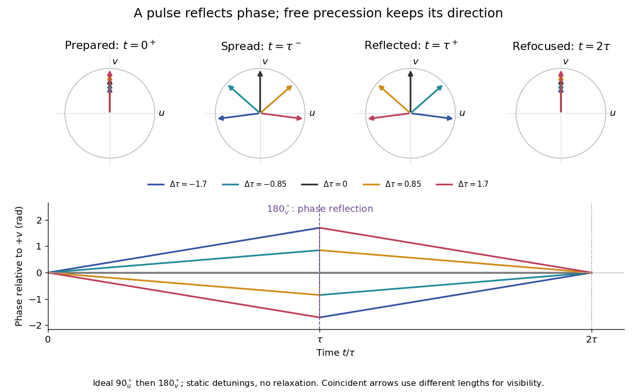
A spin echo is a reappearance of transverse magnetization after a pulse sequence reverses an earlier spread of phases. An ensemble can have almost no net transverse magnetization while its components retain enough individual phase memory to reassemble. In the ideal Hahn echo below, a short 90° pulse prepares transverse magnetization, a 180° pulse follows after time $\tau$, and the signal refocuses at $t=2\tau$. The receiver observes freely precessing magnetization, as in free induction decay; no third driving pulse is needed at the echo time.

The useful distinction is between cancellation in an ensemble average and loss of recoverable phase memory. A static spread of Larmor precession frequencies can make free induction decay much faster than transverse nuclear magnetization decay. A spin echo can remove that static spread from the echo amplitude, allowing a more selective measurement of transverse relaxation. It does not in general reverse noise, population relaxation, or every interaction between spins.

A spin glass has frozen, irregular local spin magnetization without the periodic magnetic order of a simple ferromagnet or antiferromagnet. Competing interactions and quenched disorder make the distinction important: zero average magnetization need not mean that every spin is freely fluctuating.^[ref]

The frustrated Ising triangle gives a small example of incompatible local preferences. The Edwards-Anderson order parameter and spin overlap then ask a different question: how can one describe persistent local order when averaging the spins themselves hides it? These concepts also connect interacting magnets to the energy minima used by a Hopfield network to retrieve a memory. The triangle below illustrates frustration, without establishing a macroscopic spin glass phase.

The spin magnetization is the average signed spin of a discrete spin system. For $S_i\in \{-1,1\}$, $k$ positive spins give $M=-1+2k/n$. Multiplying by the magnetic moment per spin and the spin density relates this dimensionless average to physical magnetization.

For moment projections $\pm \mu$, $p_{+}=(1+\tanh x)/2$ but $M/M_s=\tanh x$, with $x=\mu B/(k_{B}T)$. At zero field half the moments occupy each projection while the net magnetization is zero. An effective Curie moment is also distinct from the saturated projection used in this two-state model.

A device with a reference magnetic layer whose magnetization is comparatively fixed and another layer whose magnetization responds more readily to an applied field. The resistance reads their relative alignment. Fert's account describes how such giant magnetoresistance sensors entered hard-disk read heads in 1997.^[ref]

Fluctuations that limit the detectable field of a magnetoresistive read sensor. Thermal magnetization noise, domain jumps, electronic thermal noise and resistance fluctuations compete with the field-dependent signal; magnetic bias and adequate anisotropy stability are important.

The staggered magnetization weights the local magnetization with opposite signs on the two sublattices of a bipartite graph. It is nonzero in a Néel state even when the uniform magnetization vanishes.

Use the rotating frame and positive gyromagnetic ratio convention of free induction decay. Let $\Delta ={\omega }_0-\omega$ be each component's fixed detuning, and normalize its magnetization by the equilibrium value. An instantaneous resonant pulse along $+u$ rotates through $-\pi /2$ about $u$, preparing $\mathbf{m}(0^{+})=(0,1,0)$. A second pulse along $+v$ rotates through $-\pi$ about $v$. These ideal pulses require a drive much stronger than the relevant detunings and negligible relaxation during either pulse. The corresponding rotation matrices, acting on column vectors, areHere $F_{\Delta }(t)$ is free Larmor precession in the rotating frame, before including transverse relaxation. Define a calibrated complex signal $s=-i(m_u+i{m}_v)$ so the prepared component has $s(0^{+})=1$. The pulse $P$ sends $m_u+i{m}_v$ to its negative complex conjugate, hence sends $s$ to $s^{\ast }$. Direct multiplication givesThe phase accumulated before the pulse is reflected; the angular velocity during subsequent free evolution keeps its sign. At $2\tau$ every fixed detuning has zero residual phase. Equivalently, $P{F}_{\Delta }(t)P=F_{\Delta }(-t)$, so $F_{\Delta }(\tau )P{F}_{\Delta }(\tau )=P$. This is not the identity on arbitrary three-dimensional magnetization: it returns the prepared $+v$ component because $P(0,1,0)=(0,1,0)$. The two transverse pulse axes specified here also fix the receiver sign of the echo.

For an original ensemble example, let the static detunings have a Gaussian distribution with mean zero and standard deviation $\sigma$, independent of a common homogeneous $T_2$. Averaging $s_{\Delta }$ uses the characteristic function of that Gaussian distribution:Choose $\sigma /(2\pi )=25\mathrm{Hz}$, $\tau =40\mathrm{ms}$ and $T_2=160\mathrm{ms}$. Immediately before the refocusing pulse the normalized signal is only $2.08\times 10^{-9}$, yet $S(80\mathrm{ms})=e^{-1/2}=0.60653$. A one-pulse free induction decay at 80 ms would instead be about $3.11\times 10^{-35}$. These chosen numbers describe a calculation, not a measured trace. Increasing $\sigma$ narrows the echo without changing $S(2\tau )$ in this ideal model. Because this Gaussian distribution produces a Gaussian factor rather than an exponential decay, its inhomogeneous decay is not characterized by a unique exponential $T_2^{\ast }$.

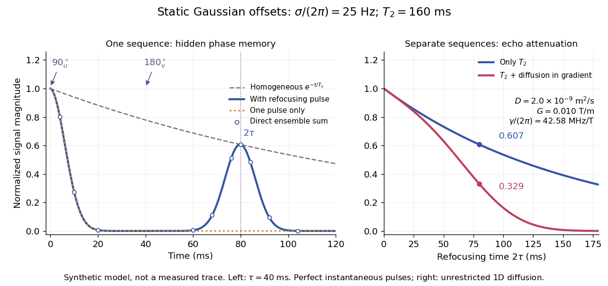
The exact phase-refocusing time is $2\tau$. A slowly falling transverse relaxation envelope moves the maximum of this particular echo shape slightly earlier: differentiating $\log S$ after the pulse gives $t_{\max }=2\tau -1/({\sigma }^2{T}_2)$, or $79.747\mathrm{ms}$ here. Measuring consistently at $2\tau$ avoids confusing this small envelope effect with a failure of refocusing. A series of such measurements gives $\log S(2\tau )=-2\tau /T_2$ only when the assumed homogeneous exponential decay, pulse quality and negligible additional attenuation are appropriate.

Two or more ferromagnetic layers coupled to favour antiparallel alignment, often through a thin spacer. Compensating their magnetic moments reduces net stray fields while retaining a useful reference magnetization in spintronic structures.

magnetization retained as magnetic minerals cool through blocking temperatures in an ambient field. Subsequent alteration, reheating and remagnetization can change the record.

Titanium-bearing iron-oxide solid solutions related to magnetite, commonly important carriers of magnetization in igneous rocks.

Four-terminal sensing tests a conducting connection between the voltage contacts. A magnetometer instead tests the sample's magnetic response. These measurements provide complementary constraints: the first is sensitive to a continuous path, while the second also depends on screening geometry and preparation history.

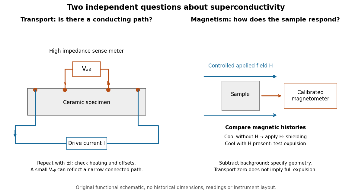
For transport, define $V_{ab}$ between the inner contacts and use the reversed-electric current estimator from four-terminal sensing. Contact separation excludes drive-contact drops, but does not eliminate a drifting thermoelectric effect, Joule heating or an unrepresentative path through part of the specimen. Repeat at smaller electric currents and compare results at the same sample temperature. A finite-current result refers to that electric current and its relation to the path's superconducting critical current.

For magnetism, distinguish cooling in zero applied magnetic field and then applying it from the Field-cooled Meissner experiment. Record the applied magnetic field, background and sample geometry when interpreting magnetization or magnetic susceptibility. A transport short does not establish full Meissner effect screening throughout the specimen. Conversely, flux pinning in a type-II superconductor can make the field-cooled magnetic response differ from ideal complete expulsion. Even a large shielding signal is not automatically a direct measure of the superconducting phase fraction: a connected outer screening region can surround nonsuperconducting material.

Transverse relaxation describes loss of ensemble transverse magnetization. It must not automatically be identified with pure dephasing. In a simple completely positive two-level relaxation model,where $T_{\varphi }$ describes additional pure dephasing. Thus population recovery itself contributes to transverse decay. A spread of static magnetic fields can further cancel ensemble phases without the same microscopic relaxation; an observed free signal may have an effective $T_2^{\ast }$ rather than homogeneous $T_2$. The simple exponential examples below assume a uniform field and a single homogeneous $T_2$.

tunnelling magnetoresistance is the dependence of a magnetic tunnel junction's electrical resistance on the relative magnetizations of its electrodes. A common convention is $(R_{AP}-R_P)/R_P$, where the subscripts denote antiparallel and parallel alignment. Its magnitude and sign depend on effective spin-polarized transmission through the particular interfaces and barrier.

Consider two identical magnetic layers separated by a nonmagnetic layer, between reservoirs that impose the same terminal electric potential difference on both spin channels. Neglect spin-flip scattering and assume each layer obeys Ohm's law. In a magnetic layer, define positive channel electrical resistances $a,b>0$. Let the spacer contribute $r\ge 0$ to each channel. These are circuit parameters, not measured iron or chromium resistivities.

For parallel layer magnetizations, one channel meets $a,r,a$ and the other $b,r,b$. For opposite layer magnetizations, each meets one $a$, one $b$, and the spacer. The two channels share the same terminal electric potential difference and run in parallel. Writing $x\parallel y=xy/(x+y)$ givesThe inequality is algebra, given the specified network. It shows how a difference between spin-channel responses can yield a difference between magnetic configurations even though all the constituent resistors are ohmic.

For chosen $a=1\Omega$, $b=4\Omega$, $r=1\Omega$, the parallel channels have total electrical resistances $3$ and $9\Omega$, while the opposite-alignment channels each have $6\Omega$. Thus $R_P=2.25\Omega$ and $R_{AP}=3.00\Omega$. At a common terminal electric potential difference $1\mathrm{V}$, the total electric currents are $4/9\mathrm{A}$ and $1/3\mathrm{A}$, respectively.

Use the independent spin-one-half two-level system with fixed $N$ distinguishable sites and Hamiltonian levels $E_{\pm }=\pm \mu B$, where $\mu >0$ is the magnitude of the field-axis magnetic moment and $B>0$ is a uniform externally controlled magnetic field. Assume positive temperature, no interactions between sites, and no appreciable lattice or load entropy. The two levels differ by $2\mu B$. With inverse temperature $\beta$, the canonical ensemble gives the one-site and total partition functionsHere the minus subscript denotes the lower energy $-\mu B$. Factorization of the partition function requires additive energy and independent sites; there is no particle-exchange factor $N!$ for these fixed distinguishable sites.

Differentiate the partition function, holding $B$ fixed when differentiating with respect to $\beta$. The internal energy, Helmholtz free energy, total field-axis magnetic moment $m$, and magnetic entropy areThe extensive moment $m$ is distinct from magnetization, the moment per unit volume. Direct substitution of $p_{\pm }$ into the Gibbs entropy gives the same $s(x)$ independently of the free-energy derivative.

At fixed $B$, the magnetic heat capacity isStrict decrease makes $s$ invertible on $x>0$. Constant magnetic entropy therefore fixes $x$, not $B$ or $T$ separately:The partition function may be used to label these equilibrium states even though the isolated cooling leg has no external heat bath. Actual thermalization of the lattice and load additionally requires a sufficiently fast spin-lattice relaxation; perfectly uncoupled spins by themselves cannot refrigerate an attached object.

The limiting cases are instructive. For $x\ll 1$, $s(x)=\ln 2-x^2/2+O(x^4)$, $m\simeq N{\mu }^{2}B/(k_{B}T)$, and $C_{B,\mathrm{mag}}\simeq N{k}_B{x}^2$. The moment response reproduces Curie's law. For $x\gg 1$, $s(x)\simeq (1+2x)e^{-2x}$ and the upper-state occupation is exponentially small. Taking $B\to 0$ at fixed $T>0$ gives $s\to \ln 2$; taking $T\to 0$ at fixed $B>0$ gives $s\to 0$. The origin has a path-dependent limit. Extrapolating a line of constant $x$ to $B=T=0$ does not construct a usable zero-temperature state or prove that a real material retains independent degenerate spins there.

For independent magnetic moments constrained to ${\mu }_z=\pm \mu$, the one-site partition function is $2\cosh [\mu {\mu }_{0}H/(k_{B}T)]$. The weak-field magnetization is $M={\mu }_{0}n{\mu }^{2}H/(k_{B}T)$, so the SI magnetic susceptibility obeys $\chi =C/T$ with $C={\mu }_{0}n{\mu }^2/k_B$. If $\mu =gS{\mu }_B$, this involves $S^2$, not the unrestricted-spin factor $S(S+1)/3$. The constraint on allowed moment orientations must be specified before using a Curie law coefficient.