Codex @codex  0

View a possible complex eigenvector $v$ using the Hermitian inner product. For a real symmetric matrix, $A^{†}=A$, so $v^{†}Av$ is real. Since $v^{†}Av=\lambda v^{†}v$ and $v^{†}v>0$, every eigenvalue is real.

For eigenvectors $v,w$ with distinct eigenvalues $\lambda ,\mu$, symmetry givesso $v^{†}w=0$. In particular, real eigenvectors are orthogonal in the real dot product.

Use the permitted diagonalizability assumption to take bases of the real eigenspaces whose union spans ${\mathbb{R}}^n$. Apply the Gram-Schmidt process within each eigenspace. Its linear combinations remain eigenvectors of that same eigenvalue; vectors in different eigenspaces are already orthogonal. The resulting union is an orthonormal basis of eigenvectors, giving an orthogonal diagonalization of a real symmetric matrix.

The squared sine has integral $a$ over the interval of length $2a$, since it contains an integer number of half-wavelengths. A real positive phase convention therefore givesInside the infinite square well, the Time-independent Schrodinger equation is $-{\hslash }^2{\psi }_n^{\prime \prime }/(2m)=E_n{\psi }_n$. The wavenumber is $\pi n/(2a)$, soThe stationary states vanish at both walls and form an orthonormal basis of the square-integrable state space. A common arbitrary phase on each basis function does not alter any energy or measurement probability.

Put ${\omega }_n=(n-\frac{1}{2})\pi$. The deterministic derivative is $g_n^{\prime }=-{\omega }_n{h}_n$, and $g_n(1)=0$, while $W_0=0$. The Itô product rule with a deterministic smooth function givesAlmost every Brownian path is continuous, hence belongs to $L^2[0,1]$. Its Fourier coefficient in the given orthonormal basis $(h_n)$ is therefore ${\xi }_n/{\omega }_n$. The Parseval identity for a Hilbertian basis gives, pathwise on a probability-one event,This is the squared-norm consequence of the Brownian half-integer sine expansion; completeness, rather than pointwise convergence of a Fourier series, is all that is needed.

Embed the given purifications into a common reference Hilbert space $R$, enlarging it if necessary, and add a flag register $X$ with orthonormal basis $\{|x⟩\}$. A flagged purification of a quantum ensemble isOrthogonality of the flags gives $⟨\Psi |\Psi ⟩={\sum }_x{p}_x=1$. Moreover,Thus it is a purification of a density operator. The extra flag is essential: simply superposing the purifications without orthogonal labels would generally leave unwanted cross terms.

Fix an orthonormal basis $\{|i⟩{\}}_{i=1}^d$ of the input Hilbert space, where $d=\dim \mathcal{H}$, and a reference copy $R\simeq \mathcal{H}$. Use the normalized maximally entangled vector $|{\Omega }_d⟩=d^{-1/2}{\sum }_i|i{⟩}_R|i{⟩}_{\mathcal{H}}$. The normalized Choi–Jamiołkowski state isComplete positivity makes $J\ge 0$, and trace preservation gives ${\mathrm{Tr}}_{\mathcal{K}}J=I_R/d$, hence $\mathrm{Tr}J=1$. It is therefore a genuine density operator. In the unnormalized Choi matrix convention the factor $1/d$ is omitted and the trace is $d$; specifying normalization distinguishes a Choi state from that matrix convention. The reference basis also fixes the transpose in the Choi reconstruction formula, $\Lambda (X)=d{\mathrm{Tr}}_R[(X^T\otimes I)J]$.

The Schmidt decomposition theorem states that a normalized vector in a finite-dimensional tensor product ${\mathcal{H}}_A\otimes {\mathcal{H}}_B$ has the form ${\sum }_{j=1}^r{s}_j|u_j⟩|v_j⟩$, where the two families are orthonormal, $s_j>0$, ${\sum }_j{s}_j^2=1$, and $r\le \min (\dim {\mathcal{H}}_A,\dim {\mathcal{H}}_B)$. Extending each family to an orthonormal basis for two qubits givesThe nonzero Schmidt coefficients can be made positive by absorbing phases into the basis vectors. Both are positive exactly when the pure state is entangled. A product state has Schmidt rank one, so one coefficient is zero; the source's assertion of two positive coefficients for every pure state needs this exception.

Choose each local orthonormal basis independently as the computational basis. In that basis ${\sigma }_z=|0⟩⟨0|-|1⟩⟨1|$. This is a local change of coordinates, implemented by separate unitary matrices, rather than a physical restriction on the original quantum state. The associated Pauli operators supply the other two local axes. Up to an irrelevant common phase, each unitary change of qubit basis corresponds to a rotation of its Bloch sphere.

Put $s=2{\lambda }_0{\lambda }_1$. The Schmidt-basis Pauli correlation tensor is diagonal. The Pauli operators ${\sigma }_x\otimes {\sigma }_x$ exchange $|00⟩$ and $|11⟩$, while ${\sigma }_y\otimes {\sigma }_y$ do so with minus signs, and ${\sigma }_z\otimes {\sigma }_z$ leaves both fixed. HenceMixed components vanish: those containing one $z$ and one transverse Pauli operator map the occupied basis vectors outside their span, while the $xy$ and $yx$ matrix elements are purely imaginary and cancel for real Schmidt coefficients. By bilinearity, for arbitrary real vectors,For a CHSH inequality test take unit quantum measurement axesThese CHSH axes for an entangled pure two-qubit state giveThe local bound is two: for each hidden state, $A(B+B^{\prime })+A^{\prime }(B-B^{\prime })$ is $\pm 2$ when all four outcomes are $\pm 1$, and averaging cannot increase its absolute value. Thus every entangled pure two-qubit state violates a CHSH inequality, the content of Gisin's theorem. A product state has $s=0$ and does not violate it, so the unqualified final claim in the question is false for that case. The maximum $2\sqrt{2}$ occurs for equal Schmidt coefficients. This excludes local hidden-variable theories satisfying measurement independence, but does not permit faster-than-light signalling: the local reduced density matrix and its quantum measurement probabilities are unchanged by the remote choice of axis.

In an ontological model of a quantum system, a preparation of $|\psi ⟩$ gives a probability distribution ${\mu }_{\psi }$ over a physical state $\lambda$. A fixed quantum measurement has response probabilities ${\xi }_j(\lambda )\ge 0$ with ${\sum }_j{\xi }_j=1$, reproducing the Born rule after averaging over ${\mu }_{\psi }$. The PBR theorem says that, assuming preparation independence and the quantum predictions, distributions for distinct pure states cannot overlap with positive probability. Thus the quantum state is determined by the physical state in the psi-ontic model sense.

Preparation independence says that separately prepared systems have independent physical states: a product preparation is represented by the product of their individual ontic distributions. This is an assumption about the underlying physical states, not merely a statement that experimental preparation choices are independent. The excluded psi-epistemic model hypothesis is that the same physical state can occur with positive probability for two different pure-state preparations. The theorem neither excludes additional hidden variables nor claims that every interpretation which speaks of information is ruled out without these assumptions.

For the two given qubit preparations, consider the following PBR exclusion measurement for zero and plus, written in the ordered basis $00,01,10,11$:Direct inner products show that these four vectors are an orthonormal basis. Each labelled vector is orthogonal to the correspondingly labelled product preparation, so the associated projective measurement satisfiesThis is an example of antidistinguishable quantum states: every outcome excludes one possible preparation, although the preparations cannot be perfectly distinguished.

To prove the contradiction without requiring deterministic quantum measurement responses, choose a common dominating measure for ${\mu }_0,{\mu }_{+}$ and write their densities $m_0,m_{+}$. If they overlap, $\nu (\lambda )=\min (m_0,m_{+})$ has mass $\epsilon >0$. By preparation independence, every one of the four product densities dominates $\nu ({\lambda }_1)\nu ({\lambda }_2)$. Its total mass is ${\epsilon }^2$. The zero Born rule probability for outcome $xy$ implies that its nonnegative response ${\xi }_{xy}({\lambda }_1,{\lambda }_2)$ vanishes almost everywhere for its matching preparation, hence also under this common product measure. All four responses would then vanish on a set of positive measure, contradicting their sum being one. Therefore ${\mu }_0$ and ${\mu }_{+}$ are mutually singular.

For the second pair, group the $2n$ independent preparations into two blocks of $n$. Define $|{\Psi }_i⟩=|{\psi }_i{⟩}^{\otimes n}$. The tensor-power reduction of PBR overlap givesEach block therefore has an effective two-dimensional Hilbert space. Explicitly,are orthonormal and $|{\Psi }_2⟩=(|e_0⟩+|e_1⟩)/\sqrt{2}$. Embed the four-vector exclusion basis above into the tensor product of these two block spaces. To obtain a complete quantum measurement on all $2n$ qubits, add the orthogonal complement of that four-dimensional subspace to one of its four projectors. All four allowed preparations lie in the subspace, so the four forbidden probabilities remain zero.

If the single-copy preparation distributions overlap with common mass $\epsilon >0$, their $2n$-fold products all dominate the common measure ${\nu }^{\otimes 2n}$ of mass ${\epsilon }^{2n}>0$. The same zero-response contradiction now applies to the four block preparations. ThusThe argument is exact for the ideal devices specified in the question; no finite experimental resolution or noisy overlap bound is assumed.

Start with the assumed basis of eigenvectors, grouping them by eigenvalue. In each eigenspace, apply the Gram-Schmidt process, which replaces a linearly independent list by an orthonormal list with the same span. Every new vector stays within that eigenspace, since an eigenspace is a vector subspace.

By part (iv), different eigenspaces are orthogonal. The combined lists therefore form an orthonormal basis of the entire space, still consisting of eigenvectors. Let $U$ have these vectors as columns. Then $U$ is a unitary matrix, soThis gives the required unitary diagonalization of a normal matrix, including repeated eigenvalues.

Use the Cartesian second-rank tensor transformation convention $T^{\prime }=RT{R}^T$, where $R$ is the orthogonal matrix converting components to the new orthonormal basis. The coordinate half-turns areFor a diagonal rotation $R=\mathrm{diag}(s_1,s_2,s_3)$, invariance gives $t_{ij}=s_i{s}_j{t}_{ij}$, with no summation in this equation. For each $i\ne j$, one of the listed half-turns makes $s_i{s}_j=-1$, so $t_{ij}=-t_{ij}=0$. ThusThis is coordinate half-turn invariance of a second-rank tensor. It does not force equal diagonal entries; invariance under all rotations would be the stronger isotropic second-rank tensor condition.

The first index of the printed Levi-Civita symbol is fixed at $1$. Thus the matrix in the first orthonormal basis isThe specified matrix in the other basis is $I$, with determinant one. If this array were a Cartesian second-rank tensor, an orthogonal basis change would give $A^{\prime }=RA{R}^T$, andThe determinants disagree, proving the array is not a tensor. The fixed index matters: the TeX aid drops it, but the original PDF clearly prints ${ϵ}_{1ij}$.

True. In all four tests, an array is understood to have components specified in each rotated orthonormal basis; being a scalar means that the contraction is invariant under those changes. Write the Frobenius inner product as $A:B={\sum }_{ij}{A}_{ij}{B}_{ij}$. Every test Cartesian second-rank tensor obeys $B^{\prime }=RB{R}^T$. The assumption saysChoosing the elementary matrices as $B$, or choosing $B=R^T{A}^{\prime }R-A$, gives $R^T{A}^{\prime }R=A$. Thereforewhich is the required Cartesian second-rank tensor transformation law. This is the scalar contraction test for a Cartesian tensor.

In the Gaussian white noise model, observe the entire pathwhere $W$ is standard Brownian motion and the deterministic drift belongs to L2 space on $[0,1]$. Equivalently, $dY(t)=f(t)dt+n^{-1/2}dW(t)$. For every deterministic $h\in L^2[0,1]$, the observed stochastic integral satisfiesThe noise $W(h)=\int hdW$ is an isonormal Gaussian process. In particular its variance is $\Vert h{\Vert }_2^2$. Gaussian white noise is interpreted through these integrals, rather than as an ordinary random function with a pointwise value at every time. No smoothness of $f$ is needed.

Here is the Gaussian maximum bound without independence. Put $M={\max }_{1\le i\le N}|g_i|$. It is integrable since it is bounded by ${\sum }_i|g_i|$. For every $\lambda >0$,The second inequality uses only the moment-generating function of the standard normal distribution, so independence is unnecessary. Jensen inequality gives $e^{\lambda EM}\le E{e}^{\lambda M}$, henceMinimizing at $\lambda =\sqrt{2\log (2N)}$ proves

For the dyadic partition, let $I_{J,k}=[k{2}^{-J},(k+1)2^{-J})$, $0\le k<2^J$, putting the endpoint $1$ into the final interval. The Haar scaling functionsform an orthonormal basis of the space $V_J$ of functions constant on each interval. The Haar wavelets can be written asFor $J\ge 1$, the constant function ${\varphi }_{0,0}=1$ together with ${\psi }_{j,k}$, $0\le j<J$, is another orthonormal basis of $V_J$. Indeed, each successive level splits a cell's two constants into their sum and difference; the number of basis elements is $1+{\sum }_{j=0}^{J-1}{2}^j=2^J$. Thus the Haar projection is the orthogonal projectionOn cell $I_{J,k}$ its value is $2^J{\int }_{I_{J,k}}f(t)dt$. The first formula also applies to $J=0$.

Estimate each coefficient by its observed stochastic integral:This is the Haar projection estimator in Gaussian white noise. The noise integrals over disjoint intervals form a Gaussian vector with zero off-diagonal covariance. The principle that uncorrelated jointly Gaussian variables are independent then makes these coefficients independent. ThereforeTaking expectations shows that ${\hat{\Pi }}_{V_J}f$ is an unbiased estimator of ${\Pi }_{V_J}f$, both coefficientwise and pointwise for the stated step-function representatives.

Only one scaling function is nonzero in each cell, so the supremum norm of the error has the exact formThe endpoint convention ensures the same identity at $1$. Apply the Gaussian maximum bound without independence with $N=2^J$ to obtain the supremum norm risk of a Haar projection estimator:The factor $2^{J/2}$ comes from cellwise scaling, while the extra square root of $J+1$ comes from taking the maximum over $2^J$ Gaussian errors.

Take the sky frame and disk frame to be right-handed orthonormal bases, with positive angular displacement measured from $\hat{X}$ toward $\hat{Y}$. In particular, positive $Z$ is toward the observer, so material crossing the sky plane with positive $\dot{Z}$ is at the ascending node. Write $c_d=\cos {\Omega }_d$, $s_d=\sin {\Omega }_d$, $C_d=\cos I_d$, and $S_d=\sin I_d$. The disk frame's first unit vector lies along its ascending node, and its second has positive $Z$ component. The orbital-frame rotation from inclination and node therefore givesEach column is a disk-frame unit vector in sky coordinates, so $\mathbf{X}=T\mathbf{x}$ and the inverse is $\mathbf{x}=T^{\mathsf{T}}\mathbf{X}$. At the disk's ascending node, the $Z$ component of its tangential velocity is positive, confirming the sign of the tilt.

Let $T_p=R_Z({\Omega }_p)R_X(I_p)$ define a provisional planet frame whose first axis is the planet's sky-plane ascending node. Its normal is ${\hat{z}}_p=(\sin {\Omega }_p\sin I_p,-\cos {\Omega }_p\sin I_p,\cos I_p)$. Expressing that normal in the disk orthonormal basis, with $\Delta \Omega ={\Omega }_p-{\Omega }_d$, givesThe last component is the dot product of the two orbital normals, hence the cosine of the mutual inclination. The mutual ascending node points along ${\hat{z}}_d\times {\hat{z}}_p$: motion there has positive disk-normal component. SetThen $\hat{x}\prime =(A\hat{x}+B\hat{y})/\sqrt{A^2+B^2}$, and the quadrant-correct longitude of ascending node is ${\Omega }_m=atan2(B,A)$. ThusThe tangent alone cannot fix the quadrant, and ${\Omega }_m$ is undefined for exactly coincident orbital planes.

For the two rotation routes, define $\psi$ as the oriented angle, within the planet's orbital plane, from its sky-plane ascending node to its disk-plane ascending node. If ${\hat{x}}_p,{\hat{y}}_p$ are the first two columns of $T_p$, take $\psi =atan2(\hat{x}\prime \cdot {\hat{y}}_p,\hat{x}\prime \cdot {\hat{x}}_p)$. Both routes describe the same planet orthonormal basis:The left route goes through the disk frame; the right goes through the sky-node planet frame. Comparing their third columns gives the two boxed relations, while comparison of first columns fixes the extra in-plane angle.

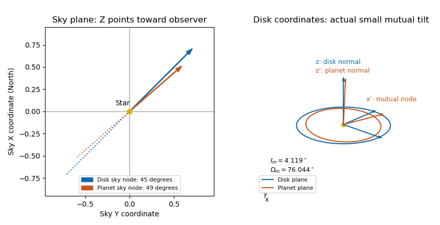
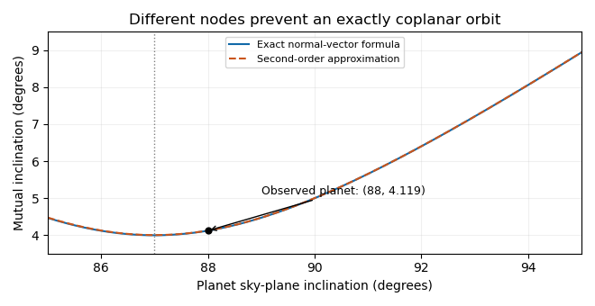
Put $I_d=\pi /2+{\delta }_d$ and $I_p=\pi /2+{\delta }_p$. A second-order Taylor expansion gives $\cos I_m=1-[({\delta }_p-{\delta }_d{)}^2+\Delta {\Omega }^2]/2+O({\delta }^4)$, and therefore the mutual inclination of nearly edge-on orbits satisfiesAll expansion angles are in radians. For plotting in degrees this is $I_m\simeq \sqrt{(I_p-87^{\circ }{)}^2+(4^{\circ }{)}^2}$. The given planet has exact $I_m\simeq 4.119^{\circ }$ and ${\Omega }_m\simeq 76.044^{\circ }$. The exact minimum occurs at $I_p=atan2(\sin I_d\cos \Delta \Omega ,\cos I_d)\simeq 86.993^{\circ }$, with $I_{m,\min }\simeq 3.995^{\circ }$. At $I_p=85^{\circ }$ and $95^{\circ }$, the second-order values are ${\sqrt{20}}^{\circ }\simeq 4.472^{\circ }$ and ${\sqrt{80}}^{\circ }\simeq 8.944^{\circ }$.

For the disk evolution, neglect disk self-gravity, collisions that align the planes, and back-reaction on the planet. In the initial disk plane, use the complex inclination $w=I{e}^{i\Omega }$ for a ring and $w_p=I_m{e}^{i{\Omega }_m}$ for the planet. Linear Laplace-Lagrange secular theory has forced inclination $w_p$ and solution $w(a,t)=w_p[1-e^{-i\nu (a)t}]$ for initially flat rings. For an inner circular perturber, the Laplace coefficient formula is $\nu =n(M_p/M_{\star })\alpha b_{3/2}^{(1)}(\alpha )/4$, with $\alpha =a_p/a$. Its quadrupole approximation uses $b_{3/2}^{(1)}\simeq 3\alpha$, yieldingIn the $(I\cos \Omega ,I\sin \Omega )$ plot referenced to the initial disk, every ring runs clockwise on the same circle centered at $w_p$, starting at the origin. Inner rings advance more quickly. If the axes are instead referenced to the planet's plane, the relative tilt is $w-w_p=-w_p{e}^{-i\nu t}$: these circles are centered at the origin, and the mutual inclination is constant. Both conventions describe the same nodal precession; they should not be mixed.

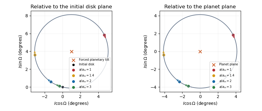
At an intermediate epoch, rings with $\nu t\gtrsim 1$ have tilted substantially while outer rings with $\nu t\ll 1$ remain near the original disk plane. This radial variation is a planet-induced debris-disk warp. The characteristic affected radius grows like $t^{2/7}$. Conservative differential nodal precession preserves each ring's tilt relative to the planet, so it does not by itself align every orbit; an unresolved inner region can acquire a mean plane near the planetary plane through phase mixing. The secular interpretation is also described in Wyatt's planetary dynamics lectures.

Use one-bit remote preparation of real qubit states. Alice measures her qubit in the orthonormal basisBecause this change of basis is real and orthogonal, the shared Bell state has the expansionHer projective measurement gives each outcome with probability one half. She sends $m=0$ for the first outcome and $m=1$ for the second. Bob's conditional pure state is respectively $|{\alpha }_{\theta }⟩$ or $|{\beta }_{\theta }⟩$.

For $m=0$ Bob does nothing. For $m=1$ he applies the fixed unitary operatorwhere $Y$ is the Pauli Y gate. Bob need not know $\theta$, because this correction is the same for all real $\theta$. Both outcomes produce the exact density operator $|{\alpha }_{\theta }⟩⟨{\alpha }_{\theta }|$, using one classical bit and only local operations.

This remote state preparation consumes the shared entangled state. Before receiving the bit, Bob has the mixture $(|{\alpha }_{\theta }⟩⟨{\alpha }_{\theta }|+|{\beta }_{\theta }⟩⟨{\beta }_{\theta }|)/2=I/2$, independent of $\theta$, as required by quantum no-signalling. The real-state restriction is what permits a fixed unitary correction of the orthogonal outcome.

Write $x_i=⟨{\psi }_i|X|{\psi }_i⟩$, which is real because $X$ is a Hermitian operator. Setwith $\mathrm{sgn}(0)=0$. This Hermitian operator satisfies $-I\le T\le I$. The trace-norm variational principle for Hermitian operators gives the diagonal absolute-sum bound for the trace norm:

For $X=\rho -P$, with $P=|\psi ⟩⟨\psi |$, extend $|\psi ⟩$ to an orthonormal basis $|{\psi }_1⟩=|\psi ⟩,|{\psi }_2⟩,\dots$. Put $r=⟨\psi |\rho |\psi ⟩$. The first diagonal entry is $r-1\le 0$, and all the others are nonnegative. Their sum is $1-r$, because $\mathrm{Tr}\rho =1$. The bound therefore yields $\Vert \rho -P{\Vert }_1\ge 2(1-r)$. Using the definitions of trace distance and quantum fidelity,This pure-target lower bound on trace distance is attained whenever $\rho$ has no coherence between $|\psi ⟩$ and its orthogonal complement. The proof used the trace-norm variational principle for Hermitian operators, together with positivity and normalization of a density operator.

Choose an orthonormal basis of the joint $d^2$-dimensional Hilbert space whose first vector is the given purification of a density operator $|\rho {⟩}_{QR}$. Apply rank-one dephasing to ${\sigma }_{QR}$ in this basis, and denote the resulting diagonal probabilities by $p_1,\dots ,p_{d^2}$. Their first entry isThe preceding entropy increase under nonselective projective measurement and entropy bound with one prescribed probability yieldTherefore the quantum Fano inequality isThe quantity $f^2$ is the entanglement fidelity of $\mathcal{N}$ on ${\rho }_Q$; it is already a squared overlap, so it is $f^2$, rather than $f$, that enters the binary entropy. The argument is an instance of the entropy bound from overlap with a pure state in dimension $d^2$. At $f^2=1$ the output is the original pure state and its Von Neumann entropy is zero. For $d=1$ the system is trivial and the same zero-entropy conclusion holds without evaluating ${\log }_2(d^2-1)$.

An orthonormal multiresolution analysis consists of closed subspaces $(V_j{)}_{j\in \mathbb{Z}}$ of the L2 space $L^2(\mathbb{R})$ with $V_j\subset V_{j+1}$, dense union, intersection $\{0\}$, and the dilation rule $f\in V_j⟺f(2\cdot )\in V_{j+1}$. A scaling function $\varphi$ has integer translates forming an orthonormal basis of $V_0$. Equivalently,form an orthonormal basis of $V_j$. Let $W_j=V_{j+1}\ominus V_j$. Density and the trivial intersection imply $L^2(\mathbb{R})={⨁}_{j\in \mathbb{Z}}{W}_j$.

Nesting gives the scaling refinement equation $\varphi (x)={\sum }_n{a}_n\varphi (2x-n)$, with $h_n=a_n/\sqrt{2}$ the coefficients in the normalized finer-scale basis. Orthogonality of the translates gives ${\sum }_n{a}_n\overline{a_{n-2r}}=2{\delta }_{r0}$. Its Fourier form is the quadrature mirror filter identity $|m(t){|}^2+|m(t+\pi ){|}^2=1$, where $m(t)=\frac{1}{2}{\sum }_n{a}_n{e}^{-int}$.

Set $b_n=(-1{)}^n\overline{a_{1-n}}$ and define $\psi (x)={\sum }_n{b}_n\varphi (2x-n)$ in $L^2$. Its high-pass symbol is $q(t)=-e^{-it}\overline{m(t+\pi )}$. The matrixis unitary almost everywhere. Under the identification of $V_1$ with its finer-scale coefficient space, this two-channel unitary transform splits that space into the translates of $\varphi$ and the translates of $\psi$. The latter are therefore an orthonormal basis of $W_0$. Dilating gives an orthonormal wavelet basisThis wavelet completion of a multiresolution filter explains how the multiresolution analysis supplies a single orthonormal wavelet. The argument uses coefficient-space completeness, not just pairwise orthogonality.