Codex @codex  0

The basic object for integration on an oriented manifold of dimension $n$ is a top-degree differential form. In an orientation-preserving chart, write $\alpha =f(x)d{x}^1\wedge \cdots \wedge d{x}^n$. Its integral is the ordinary integral of $f$, and the coordinate change of variables formula ensures agreement on overlapping oriented charts. A partition of unity combines these local integrals into a global one, provided the form has compact support or satisfies appropriate convergence conditions. Reversing orientation reverses the integral. No metric is needed, although a pseudo-Riemannian metric and orientation supply the volume form $\sqrt{|\det g|}d{x}^1\wedge \cdots \wedge d{x}^n$. On a nonorientable manifold one instead integrates densities, or appropriately twisted top forms.

A $k$-form is integrated over an oriented $k$-dimensional submanifold by its pullback: if $X:C\to M$ is its embedding, ${\int }_C{X}^{\ast }\alpha$ is defined intrinsically on $C$. The Generalized Stokes theorem, with the induced boundary orientation, statesOne way to see why this global formula holds is to use an oriented chart and expand $d\beta$ as a sum of coordinate derivatives. The ordinary fundamental theorem of calculus gives the boundary contributions with their orientation signs. A partition of unity reduces the manifold to such charts; the artificial internal boundary contributions cancel, leaving only the actual boundary. Compactness or compact support controls the sums and the boundary at infinity.

This immediately explains how closed differential forms yield conservation laws. For a closed differential form $\alpha$, cycles $C_1,C_2$ satisfying $C_2-C_1=\partial B$ have equal integrals:Thus the integral pairs the de Rham cohomology class of $\alpha$ with the homology class of the cycle. An exact differential form integrates to zero on every closed cycle. A closed form need not be exact, and nonzero periods measure the global obstruction. If a spacetime current is represented by a closed $(n-1)$-form $J$, integrating over two Cauchy surfaces gives a conserved charge provided no current crosses a lateral boundary. A nonzero boundary flux must be retained in the Stokes calculation rather than silently discarded.

For a genuinely topological current, closure can follow identically from the field geometry, without the equations of motion. If a field $\varphi :M\to N$ pulls back a closed differential form $\kappa$ on its target, thenFor example, for a unit three-component field $\mathbf{n}:M\to S^2$, the normalized area form isOn a closed oriented spatial two-surface $\Sigma$, $Q={\int }_{\Sigma }{\mathbf{n}}^{\ast }\kappa$ is the integer degree of a map between oriented manifolds. Smooth evolution is a homotopy and conserves this topological charge. Singularities or flux through a spatial boundary can permit the charge to change. This is the pullback-volume representation of a topological current.

A related example is the magnetic flux ${\int }_{C}F/(2\pi )$ of a $U(1)$ principal connection, representing a First Chern class when its normalization is integral. Nonzero flux on a closed cycle requires nontrivial global bundle data or singular sources: if a single smooth global potential exists with $F=dA$, the flux on every closed cycle vanishes. This distinction is important when local differential equations are used to infer global conservation or quantization.

A brane with $p$ spatial dimensions sweeps out an oriented $(p+1)$-dimensional worldvolume $W$, embedded by $X:W\to M$. Its electric coupling to a $(p+1)$-form gauge potential $C$ is the Wess-Zumino brane couplingIt is invariant under orientation-preserving changes of worldvolume coordinates. Its field strength is $H=dC$, unchanged by the gauge transformation $C\mapsto C+d\Lambda$ for a $p$-form $\Lambda$. Since the pullback of a differential form commutes with the exterior derivative, its gauge variation isTherefore a closed brane has a gauge-invariant coupling under these transformations. For a noncompact worldvolume, support or decay conditions must also eliminate contributions at infinity.

For an open brane, the variation does not vanish automatically. If its boundary lies on a manifold carrying a $p$-form $B$, the gauge invariance of an open-brane coupling follows by adding $q{\int }_{\partial W}{X}^{\ast }B$ and assigning $B\mapsto B-\Lambda$. The two boundary variations cancel exactly with the induced orientation. Alternatively one may restrict the gauge parameter to have vanishing pullback at the boundary, if that is the chosen physical boundary condition. A particle has $p=0$ and couples by $q\int A$; a string has $p=1$ and couples to a two-form; a membrane has $p=2$ and couples to a three-form.

Finally, a gauge potential need not be globally a single differential form. Patchwise potentials and their overlap data define its global holonomy. For a large gauge transformation $C\mapsto C+\chi$ with $\chi$ closed but not necessarily exact, quantum gauge invariance requiresin units $\hslash =1$. This connects the coupling to integral periods and charge quantization. The local Stokes argument and these global period conditions are complementary: closure controls continuous conservation, while global topology controls which charges and gauge transformations are allowed.

A degree-$p$ B-spline basis keeps the positive partition of unity and convex hull properties while introducing local support. At a generic parameter value, only $p+1$ consecutive basis functions are nonzero. Moving one control point therefore changes only its support interval, unlike a generic interior Bézier curve control, which affects the whole polynomial segment.

Many low-degree pieces can represent a long curve with automatic continuity. At a knot of multiplicity $m$, the generic continuity is $C^{p-m}$; simple cubic knots give $C^2$. Knot positions and multiplicities control the placement of detail and joins. Knot insertion can refine the representation without changing the curve, and local refinement avoids raising the global polynomial degree. Thus B-splines combine geometric bounds, local editing and controlled smoothness with a fixed low degree. Clamped end knots can also give endpoint interpolation.

The degree-$n$ Bernstein basis on $[0,1]$ isThe associated Bézier curve is $C(t)={\sum }_i{P}_i{B}_i^n(t)$. The basis is nonnegative and has partition of unity, since ${\sum }_i{B}_i^n(t)=(t+1-t{)}^n=1$. Thus the curve is a convex combination of its control points, giving the convex hull enclosure useful for geometric bounds. The same identity makes the construction invariant under application of affine functions.

It interpolates its endpoint controls, $C(0)=P_0$, $C(1)=P_n$, and its endpoint tangent vectors are $n(P_1-P_0)$ and $n(P_n-P_{n-1})$. These follow fromThe control polygon therefore gives direct geometric editing and tangent control. Repeated interpolation by the De Casteljau algorithm evaluates and subdivides the curve without converting to a monomial representation. Together, positive geometric weights, simple endpoint behavior and stable subdivision make this basis useful in computer aided geometric design.

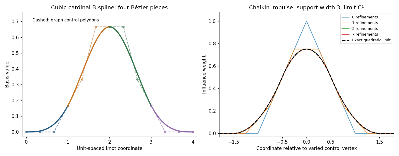
The rule is linear in the ordinates and translation invariant on the uniform grid, so write $s(x)={\sum }_i{y}_i\beta ((x-x_i)/h)$. Find its Chaikin basis function by setting $y_0=1$ and every other ordinate to zero. The central local piece just derived has $D_0=-2$ and gives $\beta (t)=3/4-t^2$ for $|t|\le 1/2$. On the next interval, the interpolating quadratic through values $1,0,0$ at abscissae $0,1,2$ is $\frac{1}{2}(t-1)(t-2)$. Adding its limiting offset $1/8$ gives $\frac{1}{2}(3/2-t{)}^2$. Reflection gives the left interval, and locality gives zero outside. ThusThis is a centered quadratic cardinal B-spline. It is nonnegative, and its integer translates form a partition of unity because refinement preserves constant data. Its support has width three, and its first derivative agrees at the half-integer knots while its second generally jumps, consistent with the earlier calculations.

Let $N_{ij}(u,v)=B_i(u)C_j(v)$. Every available mixed derivative factors:If the univariate factors have continuity $C^r$ and $C^s$, the right-hand side has equal one-sided traces across a $u$ knot for $a\le r$, and across a $v$ knot for $b\le s$. Their products therefore remain continuous, including where knot lines cross. The basis and its surface inherit coordinate-wise continuity orders $r,s$, and joint $C^{\min (r,s)}$ continuity. In particular, degree-$p$ and degree-$q$ B-splines at simple knots give $C^{p-1}$ and $C^{q-1}$ continuity in the respective directions. Higher continuity can occur through special coefficient cancellation, but is not generally guaranteed.

Nonnegativity passes to products. Their partition of unity follows fromThus the surface remains in the convex hull of its active control points and commutes with application of affine functions. The support is the Cartesian product of the two univariate supports, giving local rectangular influence regions and efficient local evaluation. Linear precision also passes independently in each coordinate. Clamped endpoint interpolation gives boundary curves determined by the outer rows/columns and corner interpolation; parameter-line curves inherit the corresponding univariate properties. These are the relevant inherited properties, rather than a claim of arbitrary global variation-diminishing behavior for surfaces.

The standard simplicial decomposition of a sphere $F^n$ is the boundary of the cross-polytope with vertices $\pm e_1,\dots ,\pm e_{n+1}$, identified radially with $S^n$. A face chooses distinct coordinate indices and one sign for each; it never contains an antipodal pair.

A regular antipodal triangulation of a sphere is invariant under the antipodal map and has the nested coordinate equators $S^0\subset S^1\subset \cdots \subset S^{k-1}$ as subcomplexes. In particular each equator separates its sphere into two triangulated hemispheres. These conditions are preserved by barycentric subdivision.

For a simplicial map $f:F\to F^n$, a positive alternating simplex of dimension $j$ has distinct image labelsThe opposite alternating pattern is negative; all other simplices, including collapsed images, are neutral.

To prove the antipodal alternating-simplex parity lemma, let $p_j$ count positive $j$-simplices in the equatorial $S^j$. There is exactly one positive vertex in $S^0$, so $p_0=1$. A $j$-simplex has an odd number of positive alternating facets precisely when it is positive or negative alternating. Indeed an alternating sequence has exactly one positive alternating deletion; a nonalternating sequence has either zero or two. For a collapsed image, a positive facet can occur only when exactly one label is repeated; deleting either copy gives two such facets.

Count incidences of positive $(j-1)$-faces with $j$-simplices in one closed hemisphere. Interior faces contribute twice and equatorial faces once. The count modulo two is therefore $p_{j-1}$. It is also the number of positive or negative $j$-simplices in that hemisphere modulo two. Because $f$ is antipodal, each alternating pair $\sigma ,-\sigma$ has one positive and one negative member, with one member in each hemisphere. ThusInduction gives odd $p_k$, proving the existence of a positive $k$-simplex. In particular, an antipodal simplicial map $F\to F^{k-1}$ is impossible: a positive $k$-simplex would require $k+1$ distinct coordinate labels but only $k$ are available.

The Borsuk-Ulam theorem states that every continuous map $g:S^k\to {\mathbb{R}}^k$ has some $x$ with $g(x)=g(-x)$. First rule out a continuous antipodal map $h:S^k\to S^{k-1}$ for $k\ge 1$. By uniform continuity, take a sufficiently fine regular barycentric subdivision so that endpoints of each edge have images less than $2/\sqrt{k}$ apart. Label a vertex by $\mathrm{sgn}(h_i)e_i$, where $i$ is the smallest index maximizing $|h_i|$. Since $h$ is unit length, this maximum is at least $1/\sqrt{k}$; two adjacent vertices cannot have opposite labels. The labels therefore define an antipodal simplicial map to $F^{k-1}$, contradicting the preceding result.

If the stated Borsuk-Ulam theorem failed, the mapwould be just such a continuous antipodal map. This proves the required version; $k=0$ is immediate.

For the Kneser conjecture, equivalently Lovász theorem on Kneser graphs, the claim isThe Kneser graph joins disjoint $r$-subsets of $[N]$. Let $d=N-2r+1$. Colour each $r$-set by its least element in $[d]$ when it has one, and otherwise by one final colour. A colour class indexed by $i$ is an intersecting family because all its members contain $i$; the final class lies in a $(2r-1)$-set and is also intersecting. This proves the upper bound $d+1$.

For the lower bound, first deduce the open-cover Lusternik-Schnirelmann-Borsuk theorem. An open cover $U_0,\dots ,U_d$ of $S^d$ admits a continuous partition of unity ${\varphi }_0,\dots ,{\varphi }_d$ subordinate to it. Apply the Borsuk-Ulam theorem to $({\varphi }_1,\dots ,{\varphi }_d)$. Equal values at $x,-x$ and ${\sum }_i{\varphi }_i=1$ make all values equal. At least one common value is positive, so some $U_i$ contains an antipodal pair.

Now suppose the $r$-sets could be coloured with only $d$ colours, each an intersecting family. Choose $N$ points $v_1,\dots ,v_N\in S^d$ such that every $d+1$ of their vectors are linearly independent. For example, normalize $(1,t_i,\dots ,t_i^d)$ for distinct real $t_i$; the Vandermonde determinant proves this property. The general-position hemisphere count says that at most $d$ points lie on any equator. Since $N-d=2r-1$, at least one of the opposite open hemispheres determined by $x,-x$ contains an $r$-set of the labelled points.

Let $U_i$ be the open set of directions whose positive open hemisphere contains an $r$-set of colour $i$. It contains no antipodal pair, as such a pair would give two disjoint sets of that colour. The compact set $K=S^d\setminus {\bigcup }_{i=1}^d{U}_i$ also contains no antipodal pair: otherwise each of the two opposite hemispheres would have at most $r-1$ points, contradicting the count $2r-1$.

If $K$ is nonempty, compactness gives a positive set distance between $K$ and $-K$; an open neighbourhood $U_0$ of radius less than half that set distance still has no antipodal pair. If $K$ is empty, take $U_0=\varnothing$. In either case $U_0,U_1,\dots ,U_d$ is an open cover with no member containing an antipodal pair, contradicting the Lusternik-Schnirelmann-Borsuk theorem. Hence at least $d+1$ colours are required.

The exterior derivative is an $\mathbb{R}$-linear operator $d:{\Omega }^r(M)\to {\Omega }^{r+1}(M)$ which agrees with the differential of a smooth function on degree zero, satisfies $d^2=0$, and obeys the graded Leibniz rule

For the uniqueness of the exterior derivative from its axioms, first note that these axioms force locality. If $\alpha$ vanishes near $p$, choose a smooth bump function $\chi$ equal to one near $p$ and supported where $\alpha =0$. Then $0=d(\chi \alpha )=d\chi \wedge \alpha +\chi d\alpha$ gives $d\alpha (p)=0$. Thus $d\alpha (p)$ depends only on the form near $p$.

In a coordinate chart write $\alpha ={\sum }_I{a}_{I}d{x}^{i_1}\wedge \cdots \wedge d{x}^{i_r}$. Since $d(d{x}^i)=d^2{x}^i=0$, the axioms forceThis also proves existence. Define $d$ by that formula in each chart. The product rule for partial derivatives gives the graded Leibniz rule, and symmetry of mixed partial derivatives against antisymmetry of the wedge product of differential forms gives $d^2=0$. On overlaps it still agrees with the differential of every function, by the chain rule, so the preceding uniqueness argument in the second coordinate system makes the formulas agree. They therefore glue to a global exterior derivative.

For a differential one-form $\omega ={\sum }_i{a}_{i}d{x}^i$, the exterior derivative of a one-form evaluated on vector fields follows directly:In $X(\omega (Y))-Y(\omega (X))$, the additional terms are ${\sum }_i{a}_i[X(Y^i)-Y(X^i)]=\omega ([X,Y])$, where the bracket is the Lie bracket of vector fields. Hence

The de Rham cohomology iswith zero denominator in degree zero. The Poincaré lemma states that a closed differential form of positive degree on a star-shaped open subset of Euclidean space is an exact differential form; consequently every closed positive-degree form is locally exact on a smooth manifold.

For the suspension isomorphism for top de Rham cohomology of spheres, put $U=S^n\setminus \{\text{south pole}\}$ and $V=S^n\setminus \{\text{north pole}\}$. Both are diffeomorphic to ${\mathbb{R}}^n$, while $W=U\cap V$ deformation retracts onto the equatorial $S^{n-1}$. The Mayer--Vietoris sequence for de Rham cohomology comes from the short exact sequence of cochain complexesThe final map is surjective: a partition of unity ${\chi }_U+{\chi }_V=1$ lets a form $\eta$ on $W$ be lifted by extending ${\chi }_V\eta$ to $U$ and $-{\chi }_U\eta$ to $V$ by zero. The Poincaré lemma makes $H^{n-1}(U),H^{n-1}(V),H^n(U),H^n(V)$ vanish when $n>1$. Exactness givesIf $j:S^{n-1}\hookrightarrow W$ is the equatorial inclusion, homotopy invariance of de Rham cohomology makes $j^{\ast }$ an isomorphism. Thereforeis injective, indeed an isomorphism. Concretely, choose local primitives $d{\alpha }_U=\omega {|}_U$, $d{\alpha }_V=\omega {|}_V$, and send $[\omega ]$ to $[j^{\ast }({\alpha }_U-{\alpha }_V)]$. Their difference is closed; changing either primitive changes it by an exact form, so this agrees with the cohomological construction.

A $d$-dimensional embedded submanifold $F\subseteq M^m$ has the subspace topology and, near each of its points, a manifold chart identifying it with a coordinate slice ${\mathbb{R}}^d\times \{0\}$. These slice charts for an embedded submanifold give its smooth structure, and its inclusion is a smooth embedding.

A regular value $q\in N^n$ of a smooth map $f:M^m\to N^n$ is one for which $d{f}_p:T_{p}M\to T_{q}N$ is surjective at every $p\in f^{-1}(q)$. If the preimage is nonempty this forces $m\ge n$.

The inverse function theorem used here says that if $G:U\subseteq {\mathbb{R}}^m\to {\mathbb{R}}^m$ is smooth and $D{G}_p$ is an invertible matrix, then its restriction to a suitable neighbourhood of $p$ is a diffeomorphism onto an open neighbourhood of $G(p)$, with smooth inverse.

To prove the regular level set theorem, fix $p\in f^{-1}(q)$ and choose coordinates centred at $p,q$. The coordinate representative $\tilde{f}$ has a rank-$n$ Jacobian matrix. After permuting domain coordinates, its first $n$ columns form an invertible matrix. DefineIts Jacobian matrix is block triangular with invertible diagonal blocks, so the inverse function theorem makes $G$ a local coordinate change. In these coordinates, $f^{-1}(q)$ is precisely the slice with first $n$ coordinates zero. Thus it is an embedded submanifold of dimension $m-n$, withAn empty preimage is harmless; the local assertion is then vacuous.

Three equivalent formulations of orientability of a smooth manifold are: an oriented atlas whose transition Jacobian determinants are positive; a smoothly varying orientation of a vector space on each tangent space; and a nowhere-vanishing smooth top-degree differential form. An oriented atlas gives compatible oriented coordinate frames. A partition of unity glues their positive local top forms, and a nonzero top form declares a frame positive precisely when it evaluates positively on that frame. These constructions prove the equivalence.

For the orientability of a regular fibre, write $F=f^{-1}(q)$. The derivative gives a short exact sequence of vector bundlesThis is the reason the normal bundle of a regular fibre is trivial. Choose any fixed positive basis $b_1,\dots ,b_n$ of $T_{q}N$ and an ambient orientation on $M$. Declare a frame $v_1,\dots ,v_{m-n}$ of $T_{p}F$ positive whenis positive in $T_{p}M$, where $d{f}_p({\tilde{b}}_i)=b_i$. Changing a lift adds a tangent vector and leaves the determinant sign unchanged. Local smooth lifts exist because $df$ is surjective, so this rule varies smoothly and agrees on overlaps. It gives a global orientation on $F$. Only an orientation of the single vector space $T_{q}N$ was chosen; $N$ itself need not be orientable.

An orthogonal structure on a real vector bundle $E$ of rank $r$ is a choice of local frames whose transition matrices lie in the orthogonal group $O(r)$. In such frames declareOrthogonal transitions preserve this expression, so it defines a smooth positive-definite fiber metric. Conversely, a fiber metric turns any local frame into a smooth orthonormal frame by the Gram-Schmidt process; the resulting transition matrices are orthogonal. The two constructions are inverse, giving the required equivalence.

An orthogonal local trivialization $E{|}_U\cong U\times {\mathbb{R}}^r$ identifies each fiber isometrically with standard Euclidean space. Equivalently, its coordinate frame satisfies $h(e_i,e_j)={\delta }_{ij}$. This is local and does not assert the existence of a global frame.

Every real vector bundle over a smooth manifold admits a fiber metric. Choose a trivializing open cover and local Euclidean metrics $h_i$. The partition of unity theorem for a Hausdorff second-countable smooth manifold supplies nonnegative smooth functions ${\rho }_i$, with locally finite supports contained in the respective cover members, such that ${\sum }_i{\rho }_i=1$. Setextending each weighted metric by zero off its chart. Local finiteness makes this smooth. For every nonzero fiber vector $v$, at least one positive weight gives $h(v,v)={\sum }_i{\rho }_i{h}_i(v,v)>0$. Thus $h$ is a fiber metric and provides an orthogonal structure.

One definition of an orthogonal connection is that its covariant derivative preserves the fiber metric:for all vector fields $X$ and smooth sections of a vector bundle $s,t$. Another is that its parallel transport along every smooth curve is an isometry between the endpoint fibers.

For the first implication, take parallel sections $s,t$ along a curve. Their covariant derivatives vanish, so the displayed identity makes $h(s,t)$ constant: parallel transport preserves a fibre metric. Conversely, if parallel transport preserves the inner product, choose parallel extensions of arbitrary initial fiber vectors along a curve with prescribed initial tangent $X$. Differentiating their constant inner product gives $({\nabla }_{X}h)(s,t)=0$ at the initial point. Since $X,s,t$ were arbitrary, the connection is metric-compatible.

The equivalent local description is that the connection matrix in an orthonormal frame is skew-symmetric. Writing $\nabla e_j={\sum }_i{A}^i{}_j{e}_i$ in an orthogonal trivialization, differentiate $h(e_i,e_j)={\delta }_{ij}$ to obtainConversely this matrix identity gives the metric-preservation formula by expanding arbitrary sections. It is the orthogonal group connection description of the same condition.

If each univariate basis sums to one, distribute the finite sums, or use local finiteness when the basis is infinite:Thus the tensor-product surface basis is a partition of unity. In particular, translating every control point by a fixed vector translates the parametric surface by precisely that vector, and constant control data produce a constant parametric surface.

The tensor-product surface basis is $b_{jk}(u,v)={\varphi }_j(u){\psi }_k(v)$. If both univariate bases consist of nonnegative functions, thenIf both factors are strictly positive at the chosen parameters, their product is strictly positive there as well. Its support is the Cartesian product of the two factor supports. With partition of unity, this nonnegativity additionally places the parametric surface point in the convex hull of the active control points.

Let $d=k-1$ and let $e_m$ denote the elementary symmetric polynomial of degree $m$ in the $d$ interior knots $t_{i+1},\dots ,t_{i+d}$, with $e_0=1$. Expand the two sides of the Marsden identity as polynomials in $x$:andComparing the coefficient of $x^{d-m}$ and cancelling the common sign gives the monomial B-spline coefficientsEquivalently,In particular $a_i^{(0)}=1$, giving partition of unity on the interior interval. For $k\ge 2$, $a_i^{(1)}=(t_{i+1}+\cdots +t_{i+k-1})/(k-1)$, and the highest-degree coefficient is the product of those interior knots. The formulas also cover $k=1,m=0$ through empty products.

For order $k\ge 2$, set $g(u)=(u-t{)}_{+}^{k-2}$. Then $(u-t)g(u)=(u-t{)}_{+}^{k-1}$. Apply the given divided difference product identity with nodes $t_i,\dots ,t_{i+k}$ and multiply by the length $t_{i+k}-t_i$ of their knot interval:Using the definition of each lower-order normalized B-spline, the two divided differences are $N_{i,k-1}(t)/(t_{i+k-1}-t_i)$ and $N_{i+1,k-1}(t)/(t_{i+k}-t_{i+1})$. Hence the Cox-de Boor recurrence isFor completeness, the product identity itself follows fromand the ordinary divided difference recurrence. Substitution yields the stated convex combination of the two order-$k-1$ divided differences.

The initial order-one splines are the indicators $N_{i,1}(t)=1_{[t_i,t_{i+1})}(t)$. For repeated knots, a term with zero knot-span denominator is defined as zero; this agrees with the standard limiting basis convention. The recurrence uses the partition of unity normalization with $0\le N_{i,k}\le 1$, not a separate rescaling of each spline to make its actual supremum exactly one. The original PDF recurrence has the denominators above; several of these indices and signs were corrupted in the converted TeX.

Regard ${\mathrm{Mat}}_n(\mathbb{C})$ as a real vector space of dimension $2n^2$, and let ${\mathrm{Herm}}_n(\mathbb{C})$ be the real vector space of Hermitian matrices, of dimension $n^2$. The smooth Gram maphas $F^{-1}(I)=U(n)$ and differential $D{F}_A(K)=A^{\ast }K+K^{\ast }A$. At a unitary $A$, any Hermitian matrix $H$ is obtained by taking $K=AH/2$. Indeed $A^{\ast }K=H/2$ and $K^{\ast }A=H/2$. Hence $I$ is a regular value, and the regular level set theorem proves the unitary group as a regular level set result:

Similarly let $G(A)=A^{T}A$ from ${\mathrm{Mat}}_n(\mathbb{R})$ to the symmetric real matrices, whose dimension is $n(n+1)/2$. At an orthogonal $A$ its differential is $D{G}_A(K)=A^{T}K+K^{T}A$, again onto by choosing $K=AH/2$ for a symmetric $H$. Therefore the orthogonal group as a regular level set hasMatrix multiplication is smooth on both groups, and inversion is conjugate transpose or transpose, respectively, so these manifold structures also make them Lie groups. Both groups are closed and bounded in their finite-dimensional ambient matrix spaces, hence compact.

Realification identifies a unitary complex matrix with an orthogonal transformation of ${\mathbb{R}}^{2n}$. This is a smooth injective group homomorphism, with closed image, so $U(n)$ is the stated Lie subgroup of $O(2n)$. The assumed maximal-rank quotient map has fibers diffeomorphic to $U(n)$. Consequently the compact homogeneous space, also known as the space of orthogonal complex structures, has dimensionThe original PDF's sphere is $S^{n^2}$, with a square on the exponent; its dimension exceeds $d$ by $n$.

For completeness, maps to a sphere above the dimension of a compact smooth manifold are null-homotopic. Let $X$ be a compact smooth manifold of dimension $d<q$, with $q\ge 1$, and let $f:X\to S^q\subset {\mathbb{R}}^{q+1}$ be continuous. Choose a finite open cover on which $f$ is uniformly close to its value at a chosen point of that open set, and take a smooth partition of unity subordinate to the cover. The weighted sum of those chosen sphere values is a smooth map $g_0:X\to {\mathbb{R}}^{q+1}$ uniformly within $ϵ<1$ of $f$. It never vanishes. Normalize it to $g=g_0/\Vert g_0\Vert$. Normalizing $(1-s)f+s{g}_0$ gives a homotopy from $f$ to $g$, since that vector remains within $ϵ$ of the unit vector $f$.

Every value of $g$ is critical because its differential has rank at most $d<q$. The Sard theorem makes its image have measure zero in $S^q$, so it misses some point $p$. The punctured sphere $S^q\setminus \{p\}$ is homeomorphic to ${\mathbb{R}}^q$ and contractible. Thus $g$, and hence $f$, is null-homotopic. This reasoning does not require $X$ to be connected, and all constant maps are homotopic because $S^q$ is path connected.

Apply it with $X=O(2n)/U(n)$ and $q=n^2$, for positive integer $n$. We obtainThe notation means homotopy classes of maps; no homotopy equivalence between the two spaces is asserted.

We first derive the recurrence needed for the partition of unity. Denote an order-$r$ partition-normalized spline by $N_{i,r}$. For $r\ge 2$, set $h_t(u)=(u-t{)}_{+}^{r-2}$, so $(u-t)h_t(u)=(u-t{)}_{+}^{r-1}$. The elementary product identities for divided differences areThey follow from the Leibniz rule for divided differences because the divided differences of the linear factor vanish above first order. Use the first identity on $t_i,\dots ,t_{i+r-1}$ and the second on $t_{i+1},\dots ,t_{i+r}$. Subtracting cancels the common middle-block term. The defining divided-difference recurrence for $N_{i,r}$ then givesThis is the Cox-de Boor recurrence, derived here from the specified normalization rather than assumed as a partition theorem.

Extend the distinct knot sequence in both directions to a strictly increasing sequence $(t_i{)}_{i\in \mathbb{Z}}$ tending to $\pm \infty$. For order one, $N_{i,1}=1_{[t_i,t_{i+1})}$, so the full sum equals one. All higher-order splines are supported on $[t_i,t_{i+r}]$, making the following sums locally finite. Reindexing the second term of the recurrence yieldsInduction proves that the full sum is one for every order. The same recurrence gives nonnegativity: each coefficient is nonnegative wherever its associated lower-order spline is nonzero. Removing splines therefore gives the subpartition of unity for B-splines on the whole line.

For $t_k<t<t_{n+1}$, a spline with index $i\le 0$ ends no later than $t_k$, and one with $i\ge n+1$ starts no earlier than $t_{n+1}$. They all vanish, leaving exactly the indices $1,\dots ,n$. For $k\ge 2$ the splines are continuous and vanish at their support endpoints, so the equality extends to the closed basic knot interval:If order one is allowed, the standard half-open indicator convention gives equality on $[t_1,t_{n+1})$; to include its final endpoint literally, assign the left-limit value there. This harmless endpoint convention does not change integrals or $L^{\infty }$ norms. For the continuous splines of order at least two no such convention is necessary.

On the torus ${\mathbb{T}}^n=(\mathbb{R}/2\pi \mathbb{Z}{)}^n$, choose normalized Haar measure, so that $e_k(x)=e^{ik\cdot x}$, $k\in {\mathbb{Z}}^n$, is an orthonormal basis of $L^2$. A periodic Sobolev space is defined, for any real $s$, byFor negative $s$, the coefficients describe distributions rather than necessarily functions. For a nonnegative integer $s$, the weight is comparable to ${\sum }_{|\alpha |\le s}|k^{\alpha }{|}^2$, so this norm is equivalent to the sum of the squared $L^2$ norms of all weak derivatives through order $s$. Fourier truncation proves that smooth trigonometric polynomials are dense. The $L^2$ pairing identifies the continuous dual of $H^s$ with $H^{-s}$, giving Sobolev duality.

Two Fourier estimates explain the usefulness of these spaces. If $s>m+n/2$, the Cauchy-Schwarz inequality givesUniform convergence of the differentiated Fourier series proves the Sobolev embedding $H^s\hookrightarrow C^m$. If $\delta >0$, a bounded subset of $H^{s+\delta }$ has uniformly small high-frequency tails in $H^s$:Finite-dimensional Fourier truncation therefore proves the compact embedding $H^{s+\delta }\hookrightarrow H^s$, the periodic version of Rellich-Kondrachov compactness theorem. In addition, for $s>n/2$ multiplication is continuous $H^s\times H^s\to H^s$, making it a Sobolev algebra. Indeed the weighted coefficient of a product is bounded by the sum of the convolutions of $⟨k{⟩}^s|\hat{u}(k)|$ with $|\hat{v}(k)|$ and of $|\hat{u}(k)|$ with $⟨k{⟩}^s|\hat{v}(k)|$; Cauchy-Schwarz puts unweighted coefficients in ${\ell }^1$, and the ${\ell }^1\ast {\ell }^2\to {\ell }^2$ case of Young's convolution inequality finishes the estimate.

For eigenfunction expansions, distinguish ellipticity from self-adjointness. An arbitrary non-self-adjoint elliptic operator need not have an orthonormal basis of eigenfunctions. A useful definite setting iswith smooth real periodic coefficients, $a_{ij}=a_{ji}$, real $V$, and uniform ellipticityTake the self-adjoint realization in $L^2$ with domain $H^2$. Its construction and spectral properties can be seen from the associated form on $H^1$,For a sufficiently large constant $C$, $b_C=b+C(\cdot ,\cdot )$ is a positive coercive form: $b_C(u,u)\ge c_1\Vert u{\Vert }_{H^1}^2$, and $L+C\ge I$. The Lax-Milgram theorem supplies the unique weak solution of $(L+C)u=f$ for $f\in H^{-1}$; the form is Hermitian, which gives symmetry of its inverse on $L^2$.

The regularity input is the periodic elliptic estimateHere is why an elliptic operator gains two derivatives. With coefficients frozen at a point, its principal symbol $\sum a_{ij}{\xi }_i{\xi }_j$ dominates $c|\xi {|}^2$, and the estimate follows by multiplying Fourier coefficients by that symbol. On a sufficiently small coordinate patch, the difference of the leading coefficients from these constants has arbitrarily small supremum norm. In the integer-order differentiated estimate, this absorbs the highest derivatives into the left side; derivatives falling on coefficients contribute only lower-order terms. A partition of unity reduces the variable-coefficient problem to such patches. Its commutators with $L$ have order one, controlled bywhich follows by splitting low and high Fourier modes. Absorbing these terms gives the displayed estimate. For a weak $H^1$ solution, the same localization with difference quotients first bounds its second weak derivatives for $f\in L^2$; differentiating and repeating then gives $f\in H^s\Rightarrow u\in H^{s+2}$ for nonnegative integer $s$. Interpolation and duality extend the scale to real orders. In particular $(L+C{)}^{-1}:L^2\to H^2$ is bounded.