A fluid particle follows a Lagrangian trajectory, so its position satisfies rather than the velocity evaluated permanently at its initial position. Assume , and writeSet and . A Taylor expansion of the velocity about givesThus , andAt the next order,so the required second-order trajectory in a sinusoidal velocity field isBoth corrections vanish at . All retained terms have units of length. The secular contribution gives the Stokes driftalthough the Eulerian time average of the given velocity is zero. The particle samples the wave at its displaced position, producing this second-order drift. The expansion is in the dimensionless parameter , for fixed times; it ceases to be uniform when the accumulated drift changes the wave phase by order unity.
Interpret “reach” first as remaining an energetic, supersonic blast wave, rather than as the arrival of any acoustic wave. An atmospheric blast-wave range estimate must account for the thin atmosphere: the distance is much greater than its height .
For an optimistic estimate, suppose the deposited energy remains in a horizontally expanding atmospheric layer. If its representative mass density is , the swept mass is of order . Conservation of energy gives the self-similar blast wave scalingUsing ordinary atmospheric estimates and speed of sound , this givesThese are scaling estimates, not an exact shock wave solution. The strong shock wave approximation would already have failed atEquivalently, keeping the disturbance strongly supersonic out to would require substantially more than the sonic-transition energy scalewhich exceeds by about a factor of twenty. Reasonable atmospheric averages and order-unity geometrical coefficients do not reverse the comparison. Escape of energy through the top of the atmosphere makes the fully confined estimate optimistic; Earth's curvature changes its area estimate by an order-unity factor.
The strong atmospheric blast will not survive to Lansing in this model. A weakened acoustic wave can nevertheless travel there. The supplied energy and atmospheric height do not determine its detectable amplitude, detailed attenuation or damage: those require an atmospheric propagation model. Thus “no disturbance of any kind reaches Lansing” would be an unjustified stronger conclusion.
This is magnetic flux freezing in ideal magnetohydrodynamics. In addition to the supplied ideal magnetohydrodynamic induction equation, a physical magnetic field obeys Gauss's law for magnetism, .
Parameterize the material surface by two particle labels , so and . Differentiating these tangents gives the material surface element evolution lawwhere . Thus the material magnetic-flux transport theorem isExpand the curl in the ideal magnetohydrodynamic induction equation:Since is the material derivative, the first three terms cancel the corresponding terms in the surface transport formula. The remaining integrand is . ThereforeNo incompressible flow assumption is needed: the changing surface area cancels the compression term. This proof assumes smooth velocity and magnetic field and a surface carried with the fluid; the ideal magnetohydrodynamic induction equation by itself, for an arbitrary non-solenoidal vector field, would leave the final divergence term.
The buoyancy frequency, also called the Brunt–Väisälä frequency, is the angular frequency of a small vertical displacement restored by buoyancy in a stably stratified fluid. Take upward, gravitational acceleration , and a background in hydrostatic equilibrium,Displace a small gas element upward by , sufficiently slowly for its pressure to match its surroundings but without heat exchange. For this adiabatic process, is constant along the element's motion, so its mass density changes by . The surrounding mass density changes by . The element's excess mass density is consequentlyIts acceleration is . ThusFor a gas of fixed composition obeying the ideal gas law, . The adiabatic buoyancy frequency of an ideal gas is thereforewhere is the specific heat capacity at constant pressure, and is the specific gas constant. Here has units ; is an angular frequency, not a cyclic frequency. Positive gives simple harmonic motion, negative gives convective instability, and is marginal. The temperature form assumes fixed composition; the preceding density form is more general.
Write the background mass density as and its hydrostatic pressure as , whereApply an Eulerian perturbation of a fluid variable to the background fields:Thus is the Eulerian pressure perturbation, in pascals; it is not the background hydrostatic pressure.
For incompressible flow, mass conservation becomes . Linearizing about rest givesThe Euler equations are . The background pressure gradient and weight cancel. Dropping products of perturbations givesUnder , replace by in inertia but retain the background mass density gradient in the displacement-induced buoyancy. This is the Boussinesq approximation. Its linear Boussinesq equations here areThe absolute value makes explicit that the small-density-variation condition concerns magnitude, including the usual negative of stable density stratification.
Use plane wave perturbations proportional to , with amplitudes . The linear equations becomeTo eliminate pressure without dividing by , multiply the vertical momentum equation by and subtract times the horizontal momentum equation:Use incompressible flow and the equation for mass density to obtain . Hence, for a nontrivial internal gravity wave,For stable density stratification, and is the buoyancy frequency. Then and the normal modes oscillate rather than grow. For , a mode with has and grows exponentially: denser fluid lies above lighter fluid. Uniform density, , is marginal for this restoring mechanism.
The case , , has zero frequency in the displayed relation. Incompressible flow then requires , so it is a degenerate non-propagating case rather than a finite-frequency vertical oscillation. These equations concern the incompressible model of part (b); its does not contain the adiabatic compression correction needed in part (a).
For , write and choose either signed branch , with . These two branches cover the roots of the squared dispersion relation. The group velocity of an internal gravity wave isIf instead the positive-frequency root is chosen for both signs of , set and multiply the displayed components by , away from the cusp .
Taking the dot product with the wave vector givesThus the group velocity, which describes the travel of a narrow wave packet and its energy, is perpendicular to the wave vector, and hence perpendicular to the phase velocity . This is the internal-wave phase and group velocity geometry. It also follows from phase-group orthogonality for degree-zero dispersion: the frequency depends only on the direction of , not its magnitude. For , the group velocity is zero, consistent with the stationary extremum .
The Rankine-Hugoniot conditions follow by integrating conservation laws across a thin moving layer, then letting its macroscopic thickness tend to zero. For example, normal momentum conservation in one dimension has the conservative formFor a shock wave moving at speed , integrate over a control interval whose endpoints move with the discontinuity. The Reynolds transport theorem giveswhere denotes the difference of limiting states. Mass conservation similarly gives . If is the normal velocity in the shock frame, combining the two relations yieldsThe same construction applied to conservation of energy, for a non-radiating normal shock wave with nonzero mass flux, gives , where is the specific enthalpy. An equation of state closes these relations, and the physical compression branch has increasing entropy.
Finite dynamic viscosity replaces the ideal discontinuity by a thin smooth transition. A viscous stress contributes a derivative to the momentum flux inside the layer and converts directed kinetic energy into internal energy. If its gradients vanish in the uniform far states, the same limiting Rankine-Hugoniot conditions still hold there. Balancing nonlinear transport with viscous diffusion gives a thickness of order in the viscous Burgers equation, where is the kinematic viscosity.
The pressure-free equation has the scalar conservation law formA smooth travelling ansatz obeys , so it cannot continuously connect two distinct constant states. The inviscid shock wave must be interpreted as a discontinuous weak solution. Its Rankine-Hugoniot condition isFor ,The result is independent of which state is called upstream. For a physical compressive entropy shock of the Inviscid Burgers equation, the left and right states satisfy and therefore : characteristic curves run into the shock wave from both sides. The ordering instead produces a rarefaction wave.
For and positive , set , so the Cole-Hopf transformation is . Substitution into the viscous Burgers equation givesHence the most general equation implied by this substitution isThe time normalization in the Cole-Hopf transformation accounts for the arbitrary function : multiplying by a nonzero function of time leaves and therefore unchanged. Replacing by sets . With this conventional normalization,the heat equation.
For each , the function obeys . By the superposition principle for this linear partial differential equation,is a solution, positive for all real . Here has units so both exponents are dimensionless. The positivity ensures that its logarithm and the resulting velocity are regular.
Let . Differentiating the logarithm givesFor definiteness order . Then dominates as , while dominates as . The limiting states areWithout this ordering convention, and . Thus the states correspond to after matching each label to its dominant exponential; the propagation speed does not depend on the naming of the two states.
Their exponent difference isConsequently, the Viscous Burgers travelling shock moves atSet and . Factoring out the mean exponential gives the hyperbolic tangent profileA precise measure of the width must be stated. The natural length in the hyperbolic tangent argument isThus the layer has thickness of order . A different common convention, jump divided by maximum gradient, gives ; the far-tail exponential e-folding length is . These differ only by their stated definitions, rather than by different solutions.
Two distinct limits require . The source permits arbitrary real constants, but in the degenerate case the solution is uniform, , and there is no shock wave or finite shock width.
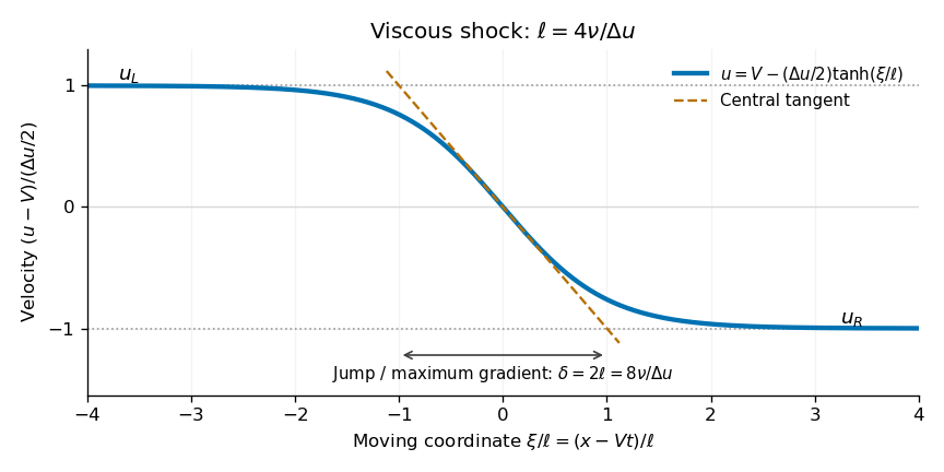
Calculated travelling shock profile and its tangent width; the horizontal coordinate moves with the shock
. Details. 
Treat the cylinder as infinitely long, with a vacuum exterior and no surface tension. Let be its gravitational potential. Integrating the gravitational Poisson equation over a coaxial cylinder of radius and length , then applying the divergence theorem, givesThus the inward gravitational acceleration is . Hydrostatic equilibrium requiresImpose zero pressure on the free surface, , and integrate inward:This is the hydrostatic self-gravitating incompressible cylinder. Its central pressure is , and the units of the expression are . A nonzero external pressure would add that constant to .
Write total pressure and gravitational potential asHere is the Eulerian perturbation of a fluid variable applied to pressure, while is the corresponding gravitational potential perturbation. They have units and , respectively. The constant interior mass density is .
The Euler equations areSubtract the hydrostatic equilibrium relation and discard terms quadratic in the perturbation. Mass conservation gives incompressible flow, and the gravitational Poisson equation has no bulk density perturbation. Thus, strictly inside the fluid,The last equation is Laplace equation, not a statement that self-gravity has disappeared. The displaced surface carries a first-order surface mass density , where is its radial displacement, and this supplies the source and matching conditions for at the moving interface. The axisymmetric gravitational potential of a displaced cylindrical interface, expressed using modified Bessel functions, incorporates that boundary source.
It is useful to define . Taking the divergence of the momentum equation gives . For an axisymmetric Fourier mode with axial wavenumber , regularity at selects radial dependence , the Modified Bessel function of the first kind, since is singular there. In what follows can always be chosen nonnegative.
Use complex amplitudes and take their real parts at the end. Write the radial surface displacement as and the combined potential asThe linear kinematic boundary condition is . Differentiate it once more in time and use the radial momentum equation, , evaluated at the unperturbed radius :With , the mode amplitudes therefore satisfyThe prime differentiates the Modified Bessel function of the first kind with respect to its dimensionless argument, rather than with respect to . The result has units , as required because is a potential. It applies to ; the uniform limit requires separate treatment.
The vanishing total pressure must be imposed at the displaced free surface, not at fixed . The first-order Taylor expansion isSince and , the Lagrangian pressure perturbation condition isThe supplied gravitational perturbation and the combined potential, evaluated at , then giveHere is the Modified Bessel function of the second kind. Equating mode amplitudes and using part (c) yieldsRearrange to obtain the dispersion relation for the axisymmetric gravitational instability of an incompressible cylinder:Every quantity on the right is dimensionless, consistent with having units . The stabilizing term comes from displacing the background hydrostatic pressure profile; omitting the Lagrangian pressure perturbation would lose it.
Define the dimensionless right-hand side of part (d) by . Then . Because and for , its sign is the sign of . The original plot is positive for sufficiently long wavelengths and negative at short wavelengths; the nonzero crossing is approximately . Numerically solving the displayed equation gives .
For , . Write with . The time factor then contains an exponentially growing solution. For , and the ideal inviscid modes oscillate stably, without damping. At the crossing the frequency is zero and the mode is marginal. In terms of the axial wavelength ,The growth rate tends to zero as , so the very longest wavelengths are not the fastest growing. The source plot has its maximum near , corresponding to and . Thus a characteristic fragmentation spacing is several cylinder diameters; a quantitative nonlinear fragment mass is beyond this linear stability calculation.
For unstable modes the physical displacement must be interpreted as with complex amplitudes handled consistently throughout. The paper's real-part notation is harmless for the squared dispersion relation, but it should not be read as imposing real in a gravitational instability calculation. The exactly uniform mode is excluded from the finite- derivation; the limit of the curve alone does not establish a separate volume-preserving uniform-radius mode.
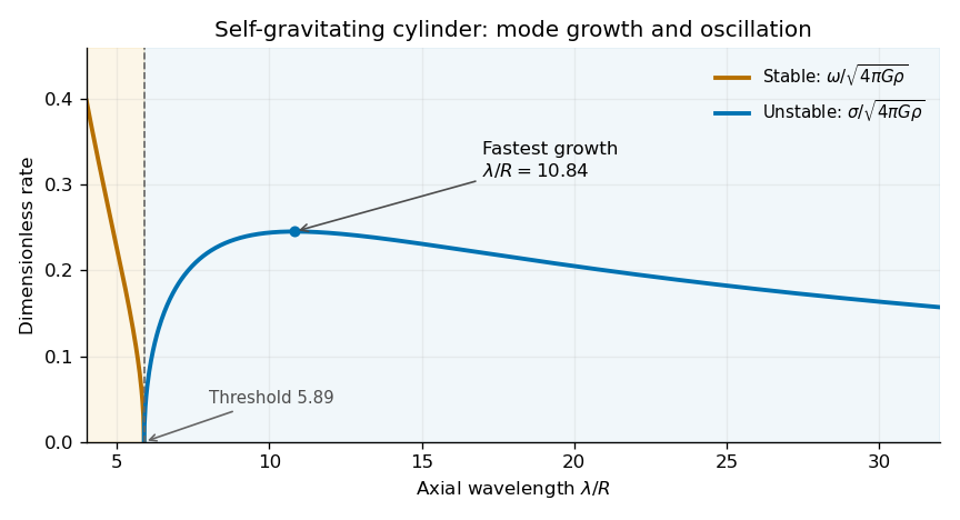
Rates computed from the cylinder dispersion relation as a function of wavelength, showing stable oscillation and unstable growth
. Details. 
Articles by others on the same topic
There are currently no matching articles.