Neither assertion holds for a general metric space. Take with and center . This is a discrete topology: both singleton sets are open and closed. The open ball is , whereas the closed ball is . Thus the interior of is , strictly larger than , and the closure of is , strictly smaller than . In general and , but the inclusions need not be equalities.
Both assertions hold for a normed vector space. The norm is continuous, so is open and is closed. If , then lies outside and converges to . Hence no such boundary point belongs to the interior of , giving . Conversely, converges to every unit vector , so . Closedness gives the reverse inclusion, and . Points already in cause no difficulty. In the zero-dimensional space , so the conclusions still hold. This is the interior and closure of norm balls; radial scaling supplies what a general metric space lacks.
Take as the semiaxis lengths. For a centered axis-aligned box with positive half-edge lengths , the volume is . Maximize under . The Lagrange multiplier equations areMultiplying by , respectively, shows that . The constraint makes each value . All boundary boxes with a zero edge have zero volume, while the positive stationary box exists. Compactness therefore gives the maximum box volume in an ellipsoidAllowing a displaced or differently oriented rectangular box cannot improve this result. Let , let be its center, and let be its perpendicular half-edge vectors. Averaging over the eight signs gives . The determinant bound , followed by the arithmetic-geometric mean inequality, makes its volume at most . The box found above attains the bound.
Let be the number of failures in mix . The total observed failures are among blocks. Equal marginal failure probabilities give , regardless of dependence within a mix. Thus the unbiased estimator based on grouped Bernoulli failure counts isFor a conventional binomial confidence interval, additionally assume independent block outcomes. Then the total has binomial distribution and the estimated standard error is . The normal approximation gives the approximate 95 percent intervalOne can instead obtain an exact, generally conservative binomial interval by solving and for the two endpoints. These equations invert binomial tail tests.
Equal marginal probabilities alone do not imply independent blocks. If the mixes are independent but blocks within a mix can be dependent, use the sample variance of the 100 counts. Here and , so . The estimated variance of is ; its standard error is , giving the large-sample interval approximately . If even between-mix independence is absent, no stated model justifies either numerical coverage claim. The estimate remains unbiased, but the uncertainty calculation needs its sampling assumptions.
The sets and are relatively open in the subspace topology on . They are disjoint and their union is . If both were nonempty, they would be a separation of , contradicting its connectedness. Therefore at least one is empty, and lies entirely in or entirely in . The assertion also holds for empty .
Let , and suppose were a separation into disjoint nonempty relatively open sets. Each connected subset lies wholly in or wholly in , by the argument just proved. Since , consecutive subsets must lie on the same side. Induction puts every on the side containing . The other side is then empty, a contradiction. Hence is connected. This is the connected chain of overlapping subsets argument; it does not require all the subsets to share one common point.
Consider a finite directed flow network with source , sink , and nonnegative finite flow network edge capacities . A feasible flow assigns to each arc and satisfies flow conservation at every vertex except . Its value is net outflow from , equivalently net inflow to . A maximal flow here means a flow of greatest value, also called a maximum flow. A source–sink cut of a flow network is a partition with , ; its cut capacity is , summing directed arcs from to its complement.
The max-flow min-cut theorem statesFor any feasible flow and cut, summing flow conservation over vertices in cancels internal arcs and gives . This proves the upper bound by every cut.
For the reverse bound, a maximum exists: the feasible set is a nonempty closed subset of the bounded product , hence compact, and is continuous. Choose a maximizing flow . Its residual network has a forward arc for unused capacity and a reverse arc for cancellable flow , retaining original-arc identities if necessary. If a residual path joined to , the minimum of its positive residual capacities would be positive. Increasing forward flows and cancelling reverse flows by this amount would preserve all constraints while increasing , a contradiction.
Let consist of vertices reachable from through positive residual arcs. Then . An original arc from to must be saturated, since otherwise its forward residual arc would make its endpoint reachable. An original arc from to must carry zero flow, since a positive reverse residual arc would again extend reachability. ThusThe upper bound and this equality prove the theorem and exhibit a residual reachability certificate for maximum flow. The argument works for real capacities and does not assume that an arbitrary augmenting-path algorithm terminates in finitely many steps.
For a linear map , its rank of a linear map is , and its nullity is . The rank-nullity theorem states . One obtains it by extending a basis of the kernel to a basis of ; the images of the added vectors form a basis of the image.
Restrict to . Its image is and its kernel is . ThusThe intersection dimension is at most , proving the lower bound. It is nonnegative, proving the upper bound by , while proves the other upper bound. Consequently the rank inequality for a composition is
In cylindrical coordinates, steady rigid rotation has , . The radial and vertical Euler equations for constant-density fluid are and , hence . Constant atmospheric pressure on the free surface gives . Conservation of fluid volume determines :ThereforeThe lowest point is the axis, where . The free surface first meets the bottom whenThis assumes no overflow and uses the full disk of wetted bottom until first contact. Once a dry central region forms, the volume constraint and geometry must be modified.
Use and its extension to square-integrable functions. For , changing variables gives . The Plancherel theorem therefore givesFor an arbitrary square-integrable , the translation identity follows by approximation by integrable square-integrable functions: translations are isometries in and the Fourier transform is continuous in the Plancherel norm. The Cauchy-Schwarz inequality makes the product on the left integrable, and is integrable on the right.
Put . Every unequal integer pair gives a nonzero integer , and every nonzero integer arises, for example with . The identity thus proves both directions of the requested equivalence. It is the orthogonality of integer translates criterion. A different Fourier normalization changes only the nonzero constant factor, not the vanishing conditions.
Work in the parent's rest frame. Momentum conservation makes the final spatial momenta equal and opposite: with magnitude . The massless energy is , while the massive energy–momentum relation is . Conservation of energy gives . Squaring and cancelling the terms givesThe two directions are arbitrary but opposite in this frame. These are total energies, including the massive daughter's rest energy, as required for relativistic two-body decay.
By equivalent norms, choose with . Differentiability in the first norm means that there is a bounded linear map with and . The same is bounded in the second norm, since . Moreover,The two norms define the same approach , so this proves differentiability with the same Fréchet derivative in the second norm. Reversing the norms proves the converse.
For completeness, the derivative is unique: if both work, fix and take . The two remainder estimates imply as , so for every . Thus differentiability and its derivative are independent of the chosen norm. This is differentiability under equivalent norms, not merely invariance of continuity.
Continuity on the compact product of unit spheres bounds the bilinear map: there is such that . This follows by scaling each nonzero vector to unit norm; if one factor space is zero, the map and the relevant assertion are trivial.
Bilinearity gives the exact expansionThe proposed derivative is linear and bounded, with . Set . Its remainder obeysThus the derivative of a continuous bilinear map is the Fréchet derivative
Take an admissible variation with at both regular endpoints. Its first variation is . Integrating the second term once and the third twice gives the boundary term , which vanishes. The fundamental lemma of the calculus of variations therefore yields the higher-order Euler-Lagrange equationHere , , and . The first two contributions cancel, leaving . For , integrate twice to obtain , and thenThe two singular-endpoint limits give and . The conditions at one give and . Hence the unique solution of the stated differential equation and limiting data isThere is a genuine distinction between solving this equation and stationarity of a finite improper action. Substitution gives , whose integral at zero diverges to . The displayed Euler-Lagrange equation remains valid for compactly supported variations on , or on regular cut-off intervals, but the literal unregularized action is not a finite stationary functional on this solution. These singular endpoints in higher-order variational problems require a regularization or an admissible-space convention if a global variational claim is intended.
A prior distribution assigns uncertainty to a parameter before observing data. Multiplying its density by the likelihood and normalizing gives the posterior distribution. A Bayes estimator minimizes the posterior expected loss function for each observed sample, and therefore minimizes integrated Bayes risk when the expectations exist.
For quadratic loss , the conditional risk is , so its minimizer is the posterior mean. For absolute loss , the one-sided derivatives or subgradients show that a minimizer is any posterior median, characterized by and .
For the stated uniform distribution sampling model, let , . The likelihood is on and zero elsewhere. Intersecting this interval with the uniform prior givesWhen , the bounded uniform-location posterior isThe posterior is symmetric, so its mean and unique median coincide. If , the data have zero marginal likelihood under the stipulated prior/sampling model and this posterior density cannot be normalized. An empty or singleton intersection is not an ordinary uniform posterior of positive width.
Use the local coordinate around infinity. A pole at is isolated: for some , is holomorphic at every point . Taking , the change of variable maps this punctured disk to . Therefore there are no finite poles outside that disk. This is a property of the local meromorphic chart at infinity, not an assertion that infinity itself is regular.
At every regular point of the Riemann sphere, there is a neighborhood containing no poles; at each pole, there is a neighborhood containing no other poles. These neighborhoods cover the sphere. Its compactness gives a finite subcover, each member containing at most one pole. Hence the total number of poles, including a possible pole at infinity, is finite. Equivalently, an infinite pole set would have an accumulation point on the compact sphere, contrary to local regularity or isolation there.
Let the finite poles be . Their Laurent series have finite principal parts . Subtracting them removes all finite singularities: is entire. Each tends to zero at infinity, so still has at most a finite-order pole at infinity.
The Laurent expansion of near has only finitely many negative powers. Thus for large , with a polynomial. The entire function is bounded outside a large disk and, by continuity, on that disk. Liouville's theorem makes it constant. ConsequentlyCombining denominators gives a rational function . This proves that meromorphic functions on the sphere are rational without assuming rationality at the start.
Write the nonconstant bijective map as with coprime polynomials and set . For a finite value , its finite preimages solve . Except for a possible leading-coefficient cancellation value, this polynomial has degree .
Multiple roots can occur only at zeros of , since at a root by coprimality. This derivative numerator is a nonzero polynomial for a nonconstant rational map. There are therefore only finitely many finite critical values to exclude. Choose outside them and outside the leading cancellation value. The fundamental theorem of algebra then gives exactly distinct finite preimages. Bijectivity forces .
Hencewhich is a Möbius transformation. Conversely, the inverse is , interpreted at its pole and at infinity, proving bijectivity on the Riemann sphere. The argument also establishes the generic-preimage interpretation of the degree of a rational map of the Riemann sphere.
First take , the hypothesis required for the printed ratios and their optimization formula to be well-defined. Since ,The maximizing and minimizing problems therefore have exactly the same solutions.
Let and minimize the separable optimization LagrangianEach summand is convex, and its derivative is . Its minimizer is . The sum of these coordinates is continuous in , decreases from infinity to zero, and is strictly decreasing wherever positive. Thus there is a unique for which the sum is . For every feasible , coordinatewise minimization gives ; both constraint terms vanish. The Lagrangian sufficiency theorem proves global optimality, not just a necessary stationary condition.
Put in decreasing order. A positive bet occurs exactly when . Hence the positive bets form an initial block. To interpret the maximal index in the question, one may include any subsequent indices tied at : their bets are zero but their marginal-return equality still holds. Take . ThenFor this block, , with the threshold inequalities determining . Zero-probability horses receive zero bets.
Let be the set attaining , and write , . For sufficiently small , the solution uses only , with there and . If the next ratio is , this remains valid when ; if all outside ratios are zero there is no finite threshold. Put . The fixed pool is , so the expected gross payout and net gain areTied best horses receive bets proportional to their existing stakes; betting all on one tied horse is not generally optimal for finite . This is pari-mutuel expected-return allocation.
The literal allowance needs qualification. At the printed objective contains and the ordered ratios are undefined. Even defining an unbacked horse's payout to be zero does not always yield an attained optimum. For example, take , , , . For , the normalized expected payout is , tending to as but never attaining it; at that zero-payout convention gives . Thus the proved allocation formula requires positive existing stakes, or an explicitly modified market model. The zero-stake case cannot be justified by silently dividing by zero.
The dual space consists of all real linear functionals on . If is a basis, its dual basis is characterized by ; explicitly extracts the th coordinate. The natural map is . It is linear and injective, because the coordinate functionals separate nonzero vectors, and both spaces have dimension . Hence it is an isomorphism. Its definition uses no choice of basis, which is the meaning of “naturally” here.
Evaluation is linear, so belongs to . For distinct nodes , define the Lagrange interpolation polynomialsThey lie in and obey . Applying a putative relation to gives , so the evaluations are independent and form a basis of . The polynomials give their dual basis in , using the canonical identification with .
Every has the interpolation expansion : the difference has distinct roots but degree at most . Integrate to get the numerical integration weights . For the specified symmetric five nodes, symmetry gives weights . Exactness on givesOdd moments vanish automatically. Solving yields Boole's rule
Use the standard constant-density incompressible flow model, with conservative body force. Write independent of , and . Differentiate the -momentum Euler equations with respect to and subtract the -derivative of the -momentum equation. Mixed pressure derivatives and the curl of a conservative body force cancel, givingThe last term vanishes by incompressibility, so the material derivative of vorticity is zero. Thus . Incompressibility is important: inviscidness alone does not suffice; in a compressible barotropic planar flow the equation is , conserving instead.
Take vortex strength to denote circulation, positive counterclockwise. A point vortex at generatesIt has zero vorticity away from its core, with circulation around the core. Each vortex moves with the other's regular induced velocity, not its own singular field. With ,Multiplication by the two strengths proves . Also , so .
For equal strengths and the specified initial positions, and . The motion of two point vortices is rotation with angular velocity :Negative circulation reverses the rotation. If vortex strength is defined instead as the coefficient of velocity, absorb the factor consistently into its definition.
Set . The complex limit at infinity gives . Parametrizing the semicircle and using yieldsBy symmetry and the supplied sine bound,The arc integral is therefore at most , tending to zero. This proves the required vanishing, the relevant form of Jordan's lemma. No holomorphicity of is required just for this arc estimate.
Integrate around the positively oriented indented upper-half-plane contour. The outer semicircle runs from to ; the inner semicircle runs clockwise from to , excluding zero. The integrand is holomorphic inside this region, so Cauchy's integral theorem gives total integral zero.
The outer arc tends to zero by part (a) with and . On the inner arc , decreases from to zero, andThe two real segments combine asPassing to the limits gives , and hence the Dirichlet integralThis is an ordinary conditionally convergent improper integral: the integrand tends to one at zero, and integration by parts gives a tail bounded by beyond . The clockwise indentation sign is essential.
The Lorentz factor is . Length contraction makes the moving javelin's length in the shed frameThis measures its two endpoints at the same shed-frame time.
The shed moves relative to the javelin frame at the same speed, so its simultaneous length there isThe javelin retains its proper length . The two statements use different simultaneity slices, as prescribed by relativity of simultaneity.
Choose event , when the trailing end reaches the entrance, as and as the primed origin. Write , . Before impact, the shed-frame worldlines are entrance , back , trailing end , and leading end . The Lorentz transformation isThus in the javelin frame the ends have and , while the entrance and back have and . These four lines in each frame produce the requested spacetime diagrams. The diagrams show initial motion; dashed portions extrapolate that motion beyond first impact and are not a model of collision dynamics.
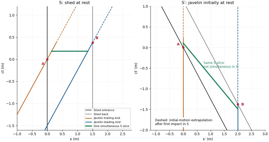
Javelin and shed worldlines in both inertial frames, with entrance event A, first impact B and a simultaneous shed-frame containment slice
. Details. 
In the shed frame, the leading end reaches the back when , giving . Transforming both events yieldswith every coordinate in metres. The invariant interval isThus the events are spacelike separated. Event occurs first in the shed frame, but occurs first in the javelin frame; this is allowed for spacelike separation.
In the shed frame there is a pre-impact interval during which both ends lie inside the shed, since its simultaneous moving length is only . Those simultaneous endpoint events do not remain simultaneous after a boost. In the javelin frame the front hits the back before the rear enters, and there is no simultaneous pre-impact containment of the full rod in a shed. This is rod containment and simultaneity, not inconsistent length measurements.
After impact, the front's motion changes while the rear cannot respond instantaneously: stress signals propagate no faster than light. A claim that the entire javelin stops rigidly at event is inadmissible. Actual post-impact compression or fracture needs material data and is not represented by the straight-line extrapolations in the diagrams.
Articles by others on the same topic
There are currently no matching articles.