Past exam of the mathematics course of the University of Cambridge / 2002 / ib

No. Consider the triangular functions $f_n(x)=\max (1-n|x|,0)$. The absolute-value and positive-part maps are Lipschitz continuous, so $|f_n(x)-f_n(y)|\le n|x-y|$. Each $f_n$ is therefore uniformly continuous on the whole real line. For $x=0$ its value is always one; for every fixed $x\ne 0$ it eventually vanishes. Hence its pointwise limit isThis limit is not continuous at zero: along $x_j=1/j\to 0$, $f(x_j)=0\nrightarrow 1=f(0)$. Individual uniform continuity does not provide a modulus uniform in $n$.

Yes; in fact the limit is uniformly continuous. Given $\epsilon >0$, uniform convergence provides one $N$ with ${\sup }_x|f_N(x)-f(x)|<\epsilon /3$. Uniform continuity of this particular $f_N$ provides $\delta >0$ such that $|x-y|<\delta$ implies $|f_N(x)-f_N(y)|<\epsilon /3$. The triangle inequality then givesThis same $\delta$ works at every point of $\mathbb{R}$, proving uniform continuity and therefore continuity. The use of one global $N$ is exactly what fails for mere pointwise convergence.

The Fourier sine series has coefficientsby integration by parts. ThusIts odd extension is $x$ on $(-L,L)$, continued with period $2L$. The usual Fourier convergence result for a piecewise smooth periodic function gives the value at a continuous point and the mean of one-sided limits at a jump. At $x=3L/2$, subtracting one period gives $-L/2$, a continuous point of this extension. Therefore the sine series converges to $-L/2$ there.

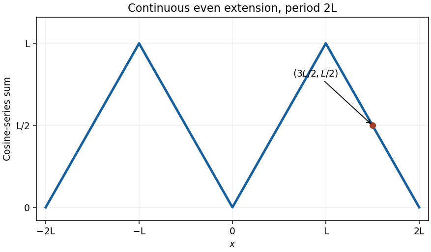
For the Fourier cosine series, the even extension is $|x|$ on $[-L,L]$, continued with period $2L$. Its triangular wave is continuous even at the joining points, so the cosine series converges to that extension everywhere. On the requested interval its graph isThe vertices are $(-2L,0),(-L,L),(0,0),(L,L),(2L,0)$. In particular, its value at $3L/2$ is $L/2$.

For a dominated family of sample distributions, a statistic $T$ is a sufficient statistic precisely when the probability mass function or density factors aswhere $h$ does not depend on the parameter. This is the Fisher-Neyman factorization theorem.

Here is the discrete proof in both directions. Suppose the factorization holds, and write $H(t)={\sum }_{x:T(x)=t}h(x)$. Then ${\mathbb{P}}_{\theta }(T=t)=g_{\theta }(t)H(t)$. Whenever this probability is positive, $H(t)$ is finite and positive andis independent of $\theta$. Thus the conditional distribution of the whole sample given $T$ is parameter-free, which is the definition of a sufficient statistic.

Conversely, if $T$ is sufficient, let $q_t(x)$ denote this common conditional mass function on each possible fiber. ThenTake $g_{\theta }(t)={\mathbb{P}}_{\theta }(T=t)$ and $h(x)=q_{T(x)}(x)$ to obtain the factorization. Fibers impossible for every parameter can be assigned $h=0$; conditional probabilities are required only for fibers with positive probability.

For the independent Poisson sample the joint mass function isAll parameter dependence is throughso this is a one-dimensional sufficient statistic. The sample mean contains the same information, since $n$ is known.

Let $G$ be the finite group and choose a point $p$. Its orbit $E=\{gp:g\in G\}$ is a nonempty finite set. Every group element permutes $E$ and maps a closed metric disc onto a disc of the same radius. By the permitted uniqueness of the smallest enclosing disc, it fixes that disc and therefore its centre $o$. Thus $G$ lies in the orientation-preserving stabilizer of one point.

In the Euclidean plane, translate $o$ to zero. Every isometry fixing zero is an orthogonal linear map: distance preservation gives preservation of inner products by the polarization identity, and its values on an orthonormal basis then determine the linear map. Orientation preservation gives determinant one, so it is a rotation. Consequently $G$ embeds in the circle group of rotation angles.

For the hyperbolic plane, use this precise standard fact about its isometries: after placing a point at the origin of the Poincare disc model, every orientation-preserving isometry fixing it has the form $z\mapsto e^{i\theta }z$. Equivalently, its point stabilizer is the rotation group, and its action on directions at the point is faithful. This is a general hyperbolic-plane fact allowed by the question. It again identifies $G$ with a finite subgroup of the circle group.

Finally, a nontrivial finite rotation group has a least positive angle $\theta$ in $[0,2\pi )$. Divide any other angle $\varphi$ by $\theta$: the remainder $\varphi -k\theta$ is another group angle in $[0,\theta )$, so it must be zero. Similarly the remainder of $2\pi$ is zero, and $\theta =2\pi /m$ for an integer $m$. The rotation through $\theta$ generates the group. The trivial group is cyclic as well. Therefore both finite orientation-preserving plane isometry groups are cyclic. This proves the finite orientation-preserving plane isometry groups are cyclic result using the same enclosing-disc argument in both geometries.

Relative to the coordinate basis, the linear map has matrixExpanding $\det (tI-F)$ in its first column gives the monic characteristic polynomialIts eigenvalues are $1$ and $(1\pm i\sqrt{7})/2$, three distinct complex numbers. Eigenvectors corresponding to distinct eigenvalues are linearly independent, so they form a basis of ${\mathbb{C}}^3$ and $f$ is diagonalizable.

Every annihilating polynomial must vanish at all three eigenvalues: applying $p(f)$ to a corresponding eigenvector gives $p(\lambda )v$. Conversely, in the eigenbasis the product of the three distinct linear factors annihilates $f$. Hence the minimal polynomial isIf $af+b{f}^2=0$ with scalars $a,b$ not both zero, the nonzero polynomial $at+b{t}^2$ of degree at most two would annihilate $f$, contradicting this minimal degree of three. Thus $f$ and $f^2$ are linearly independent endomorphisms.

The divergence is ${\partial }_x(kty)+{\partial }_{y}0+{\partial }_{z}0=0$, so this is an incompressible flow. With the planar convention $(u,v)=({\psi }_y,-{\psi }_x)$, one stream function isAt a fixed nonzero $kt$, the streamlines have $y=\mathrm{constant}$ and $z=\mathrm{constant}$, since the instantaneous velocity is purely axial. If $kt=0$, every point is instantaneously stationary and there is no distinguished streamline direction.

Follow a marked particle initially at $(0,y_0,0)$. Its trajectory satisfies $\dot{y}=\dot{z}=0$ and $\dot{x}=kt{y}_0$, soThese points form a straight segment on $x=(k{t}^2/2)y$, $z=0$, not an instantaneous horizontal streamline. Its length isThe directed angle of its vector from the origin to the marked endpoint isFor $k>0$ and $t>0$, this is $\arctan [2/(k{t}^2)]$; it equals $\pi /2$ at $t=0$. If an unoriented acute angle to the axis is intended, use $\arctan [2/(|k|t^2)]$, with $\pi /2$ when $kt=0$. This distinction handles a negative value of the given constant as well. If $a=0$, the marked set is a single point: the length formula gives zero and no line direction is defined.

Fix real $y$ and use a rectangle with vertical sides at real coordinates $\pm R$. The function $e^{-z^2}$ is entire, so its closed contour integral is zero by Cauchy's integral theorem. The bottom horizontal side contributes ${\int }_{-R}^R{e}^{-x^2}dx$ and the top contributes the negative of ${\int }_{-R}^R{e}^{-(x+iy{)}^2}dx$. This identity applies for either sign of $y$, with the corresponding oriented rectangle.

On a vertical side, $z=\pm R+is$ with $|s|\le |y|$, andThe sum of the two vertical integrals in absolute value is at most $2|y|e^{-R^2+y^2}\to 0$. Both horizontal improper integrals converge absolutely, since $|e^{-(x+iy{)}^2}|=e^{y^2}{e}^{-x^2}$. Letting $R\to \infty$ therefore provesComplete the square in the Fourier transform:The shifted-integral identity applies after scaling by $\sqrt{2}$. The Gaussian integral is $\sqrt{2\pi }$: the square of $\int e^{-u^2}du$ becomes $2\pi {\int }_0^{\infty }{e}^{-r^2}rdr=\pi$ in polar coordinates. Thus the Gaussian Fourier transform yieldsThe eigenvalue reflects the unnormalized transform convention in this question.

For a real symmetric bilinear form, a basis puts its quadratic expression in diagonal form with $p$ positive, $q$ negative and $r$ zero squares. Its rank is $p+q$, the rank of the coefficient matrix, or equivalently the codimension of its radical. Its signature is $p-q$; the signature pair is $(p,q)$, another common convention.

These quantities do not depend on the basis. A basis change replaces the matrix $M$ by $P^{T}MP$ with $P$ invertible, preserving matrix rank. The number $p$ is intrinsically the largest dimension of a subspace on which the form is positive definite. In a diagonal representation the positive coordinate space attains this dimension; any subspace of dimension greater than $p$ intersects the negative-plus-null coordinate space nontrivially and therefore cannot be positive definite. The same argument with signs reversed characterizes $q$. This proves the needed invariance, rather than assuming it from a chosen representation.

Decompose the full matrix space asusing the symmetric traceless, skew-symmetric and scalar parts. The summands are orthogonal for the given form. Indeed $\mathrm{tr}(SK)=0$ for symmetric $S$ and skew-symmetric $K$, by transposition and cyclic invariance of trace, while both non-scalar summands are traceless and hence orthogonal to $I$. On them,for nonzero vectors in their respective summands. The dimensions are $n(n+1)/2-1$, $n(n-1)/2$ and one. Therefore the modified trace form on real matrices hasThere is no radical for $n\ge 2$.

A normalizable bound state has $0<E<V_0$: the potential is nonnegative, while exponential decay is needed on the infinite right-hand region. Set $k=\sqrt{2mE}/\hslash$ and $\kappa =\sqrt{2m(V_0-E)}/\hslash$. The hard-wall condition and decay selectContinuity at $a$ has already been used. Since the finite step contains no delta interaction, integrating the Schrödinger equation across it also requires derivative continuity. Thus $k\cos (ka)=-\kappa \sin (ka)$, givingThe ground-state solution uses the first branch $\pi /2<ka<\pi$ and has no internal node. It starts at zero, rises to one maximum inside the well, decreases to a positive value at $a$, and joins smoothly onto a decaying exponential tail.

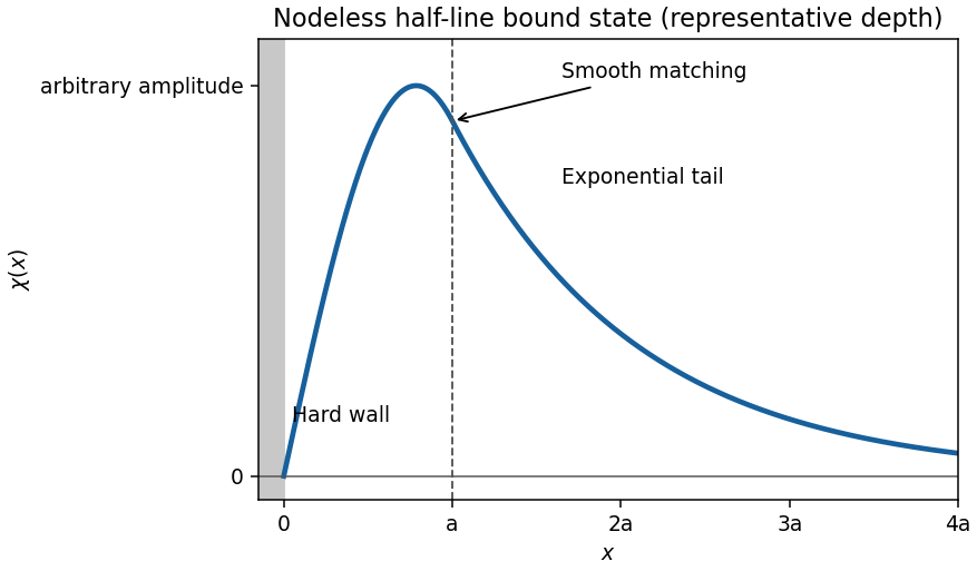
To see the precise existence condition, set $z=ka$ and $K=a\sqrt{2m{V}_0}/\hslash$. The first-branch matching equation gives $K=z/\sin z$ on $\pi /2<z<\pi$. This increases strictly from $\pi /2$ to infinity, since its derivative is $(\sin z-z\cos z)/{\sin }^{2}z>0$. Thus the bound ground state exists exactly when $a\sqrt{2m{V}_0}/\hslash >\pi /2$, or $V_0>{\pi }^2{\hslash }^2/(8m{a}^2)$, as in the bound-state thresholds for a square well with one hard wall. At equality $\kappa =0$ and the exterior solution is not square-integrable. Below it there is no normalizable energy eigenfunction of the requested ground-state type. The sketch assumes the binding condition and uses one representative solution, not a specified numerical well depth.

Take any sequence $(y_n)$ in $Y$. Surjectivity lets us choose $x_n\in X$ with $f(x_n)=y_n$. By sequential compactness of $X$, some $x_{n_j}\to x\in X$. Continuity gives $y_{n_j}=f(x_{n_j})\to f(x)\in Y$. Thus $Y$ has the Bolzano–Weierstrass property.

Now suppose $f$ is a bijection. To prove continuity of its inverse, let $y_n\to y$ and put $x_n=f^{-1}(y_n)$, $x=f^{-1}(y)$. If $x_n\nrightarrow x$, there are $\epsilon >0$ and a subsequence with $d(x_{n_j},x)\ge \epsilon$. Sequential compactness supplies a further subsequence converging to $x^{\prime }$. By continuity of $f$, $f(x^{\prime })=\lim y_{n_j}=y=f(x)$. Injectivity implies $x^{\prime }=x$, contradicting the fixed lower distance bound. Hence $x_n\to x$. Sequential continuity is equivalent to continuity in metric spaces, proving $f^{-1}$ is continuous.

Apply this to $g(t)=e^{it}$ on $[-\pi /2,\pi /2]$, mapping onto the closed right semicircle $S$. This interval is sequentially compact, and $g$ is a continuous bijection: two equal exponential values differ by an integral multiple of $2\pi$, impossible for distinct points of an interval of length $\pi$. Consequently $g^{-1}:S\to [-\pi /2,\pi /2]$ is continuous. For $\mathrm{Re}z>0$, the normalization $z\mapsto z/|z|$ is continuous and takes values in the open right semicircle. Thereforeis a continuous argument satisfying $z=|z|e^{i\mathrm{Arg}z}$. Equivalently it is $\arctan (\mathrm{Im}z/\mathrm{Re}z)$.

Put $\mu =\cos \vartheta$ and separate $\Phi =R(r)Y(\mu )$. Multiplying Laplace's equation by $r^2/(RY)$ givesFor the regular polynomial angular modes, $\lambda =n(n+1)$ and $Y=P_n(\mu )$ is a Legendre polynomial. The radial equation has branches $r^n$ and $r^{-n-1}$. Regularity at the origin keeps only the first inside, and decay at infinity keeps only the second outside. Continuity at $r=1$ identifies their coefficients, so a mode hasIts outward-minus-inward radial derivative is $-(2n+1)a_n{P}_n(\mu )$. The prescribed angular dependence decomposes as $V{\mu }^2=V{P}_0/3+2V{P}_2/3$, since $P_0=1$ and $P_2=(3{\mu }^2-1)/2$. Hence $a_0=-V/3$ and $a_2=-2V/15$, with no other required modes. The spherical harmonic matching with a derivative jump givesBoth branches are harmonic in their respective regions. They agree at the sphere, and their derivative jump is $V/3+(2V/3)P_2=V{\cos }^2\vartheta$. The interior is regular at zero and the exterior decays at infinity. An additional homogeneous matching mode would satisfy $-(2n+1)a_n=0$, so its coefficient vanishes.

Treat the two row totals as fixed sample sizes, with independent multinomial observations within each row. More generally let $N_{ij}$ be an $r$ by $c$ table, row totals $n_i$, column totals $m_j$ and total $N$. Under the unrestricted alternative, row $i$ has its own category probabilities $p_{ij}$; independence means that all rows have the same probabilities $p_j$.

Ignoring the multinomial coefficients, which cancel in a likelihood ratio, the unrestricted likelihood is ${\prod }_{ij}{p}_{ij}^{N_{ij}}$. Maximizing ${\sum }_j{N}_{ij}\log p_{ij}$ under ${\sum }_j{p}_{ij}=1$ gives ${\hat{p}}_{ij}=N_{ij}/n_i$. Under the null, the log likelihood is ${\sum }_j{m}_j\log p_j$, giving ${\hat{p}}_j=m_j/N$. Thus the null fitted counts are $E_{ij}=n_i{m}_j/N$, and the generalized likelihood ratio isA zero observed count contributes zero by continuity. Small $\Lambda$, equivalently large $G^2$, is evidence against independence. The unrestricted model has $r(c-1)$ free probabilities and the null has $c-1$, a difference of $(r-1)(c-1)$. Under the usual large-sample likelihood-ratio approximation at an interior null, $G^2$ has a chi-squared distribution with that many degrees of freedom. This is the likelihood-ratio test of independence in a contingency table. Sampling the entire table multinomially instead gives the same statistic and degrees of freedom after estimating the row probabilities.

For the supplied data the fitted counts areSubstitution givesThere are $(2-1)(3-1)=2$ degrees of freedom. The supplied 1% critical value is $9.21$, and $0.9701<9.21$. Do not reject independence at the 0.01 level. The approximate chi-squared tail probability is $e^{-G^2/2}\simeq 0.616$. This lack of rejection does not establish that the classifications are independent; the test supplies no evidence against that null here. All fitted counts are at least ten, making the stated asymptotic approximation reasonable.

For $g(z)=(az+b)/(cz+d)$ with real coefficients and $ad-bc=1$, direct subtraction from its conjugate givesThe imaginary part remains positive, and the inverse transformation has the same form, so $g$ is a bijection of the upper half-plane. MoreoverThus every path has the same hyperbolic length as its image. Taking the infimum over connecting paths, and using the inverse for the reverse inequality, proves every $g\in \Gamma$ is an isometry.

LikewiseIts squared modulus and the two imaginary-part factors cancel in the quotient, proving

We can normalize any ordered distinct pair to $(i,iy)$ with $y>1$. First send $z=x_0+i{y}_0$ to $i$ by $(\zeta -x_0)/y_0$, a real determinant-one Möbius transformation after rescaling its representing matrix. The stabilizer transformationsfix $i$. Under the Cayley map $C(\zeta )=(\zeta -i)/(\zeta +i)$, direct substitution gives $C(k_{\tau }\zeta )=e^{2i\tau }C(\zeta )$. Choose $\tau$ to rotate the second point's nonzero disc coordinate onto the positive real axis. Its inverse image is $iy$ with $y=(1+|C|)/(1-|C|)>1$.

The vertical path from $i$ to $iy$ has length $\log y$. Any other path has length at least $\int |dy|/y\ge |\int dy/y|=\log y$, so $\rho (i,iy)=\log y$. ConsequentlyInvariance of both quantities transfers this equality back to every pair; coincident points satisfy it as well. Therefore

For the right-triangle identity, normalize its right vertex to $i$ and one leg to the vertical geodesic, with endpoint $iy$, $y>1$. The other leg lies on the unit semicircle, with endpoint $s+it$, $s^2+t^2=1$, $t>0$. These geodesics meet orthogonally at $i$, since the metric is conformal to the Euclidean metric. The semicircle is a geodesic because a real Möbius transformation sends it to a vertical line; vertical lines are minimizing by the same length bound. The stabilizer rotations above can align any given tangent direction, giving this normal form for every right triangle.

If the legs have lengths $a,b$ and the opposite side has length $c$, the distance formula givesandThus the hyperbolic Pythagorean theorem is

After choosing a basis of $V$, a linear endomorphism is specified by an $n$ by $n$ matrix, with $n^2$ freely chosen coefficients. ThereforeThe $n^2+1$ endomorphisms $I,\alpha ,\dots ,{\alpha }^{n^2}$ are linearly dependent. Some nonzero coefficient list gives a nonzero polynomial $p$ satisfying $p(\alpha )=0$.

For nonzero $V$, the minimal polynomial $m_{\alpha }$ is the monic polynomial of least degree annihilating $\alpha$. It is unique: subtracting two monic least-degree choices would give a lower-degree annihilator. More generally division of any annihilator $p$ by $m_{\alpha }$ gives $p=q{m}_{\alpha }+r$, with $\mathrm{deg}r<\mathrm{deg}{m}_{\alpha }$, and evaluation implies $r(\alpha )=0$. Minimality forces $r=0$, so every annihilator is divisible by $m_{\alpha }$. If $V=\{0\}$, the convention $m_{\alpha }=1$ handles the degenerate case.

The arguments work over the underlying scalar field. In part (b), roots in that field correspond to eigenvalues there; to discuss other roots one extends scalars, for example by complexifying a real vector space.

If $\alpha v=\lambda v$ with $v\ne 0$, then $m_{\alpha }(\alpha )v=m_{\alpha }(\lambda )v$. The left side vanishes, so $m_{\alpha }(\lambda )=0$.

Conversely, if $m_{\alpha }(\lambda )=0$, write $m_{\alpha }(X)=(X-\lambda )q(X)$. Then $(\alpha -\lambda I)q(\alpha )=0$. If $\alpha -\lambda I$ were invertible, multiplying by its inverse would imply $q(\alpha )=0$, contradicting the minimal degree. Thus $\alpha -\lambda I$ is not invertible. In finite dimension this means it has a nonzero kernel, furnishing an eigenvector with eigenvalue $\lambda$. Hence the eigenvalues are exactly the roots of the minimal polynomial, with the scalar-field convention stated in part (a).

Invariance of $W$ means every power of $\alpha$ restricts to the corresponding power of $\beta$. Therefore $m_{\alpha }(\beta )$ is the restriction of $m_{\alpha }(\alpha )$, and it is zero. Divide $m_{\alpha }=q{m}_{\beta }+r$ with $\mathrm{deg}r<\mathrm{deg}{m}_{\beta }$. Evaluation at $\beta$ gives $r(\beta )=0$. By minimality of $m_{\beta }$, $r=0$, provingThe zero-subspace case has $m_{\beta }=1$ and satisfies the same conclusion.

Take $V={\mathbb{R}}^3$, $\alpha =\mathrm{diag}(0,1,0)$ and $W=\mathrm{span}(e_1,e_2)$. Then $W$ is a proper invariant subspace, and the restriction has matrix $\mathrm{diag}(0,1)$. In each case $X(X-1)$ annihilates the operator, while any annihilator must vanish at both zero and one. ConsequentlyThis same example works over any scalar field.