Past exam of the mathematics course of the University of Cambridge / 2011 / ia / Paper 2 / Section II

Combine the real variables into $z=x+iy$. The linear system of ordinary differential equations becomes $z^{\prime }=(1-i\mu )z$, hence $z=(A+iB)e^{(1-i\mu )t}$ for arbitrary real $A,B$. Taking real and imaginary parts givesThe two independent constants cover every real initial condition. In the phase plane, the distance from the origin grows as $e^t$ and the polar angle changes at rate $-\mu$. For $\mu \ne 0$ the trajectories are outward logarithmic spirals; for $\mu =0$ they are outward straight rays.

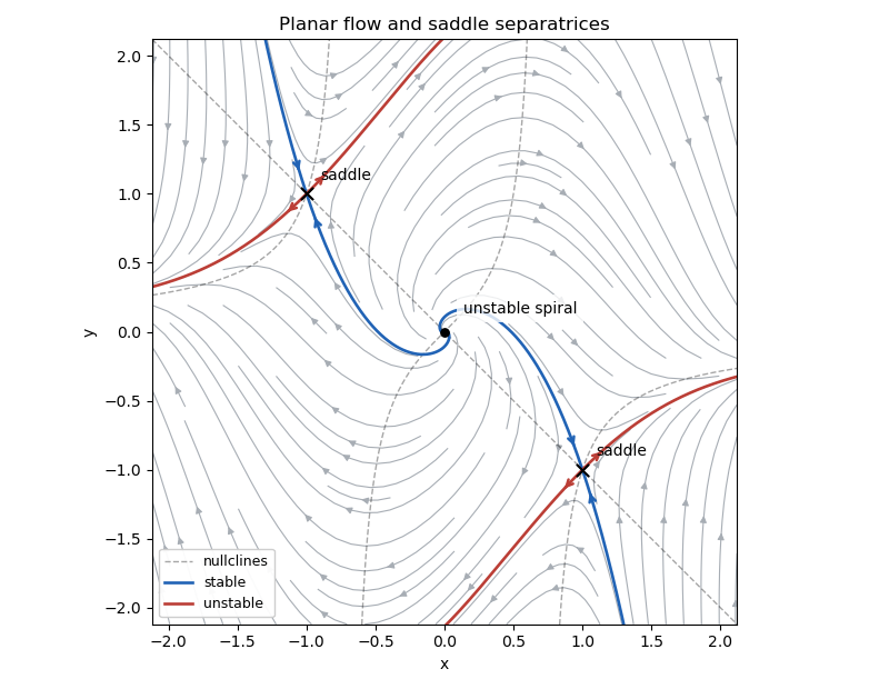
At a fixed point, the first equation gives $y=-x$. Substitution into the second gives $2x(x^2-1)=0$, so the equilibrium points are $(0,0),(1,-1),(-1,1)$. The Jacobian matrix isAt the origin its eigenvalues are $1\pm i$, so the origin is an unstable spiral. The local rotation is clockwise: on the positive $x$-axis the velocity points downward. At either nonzero equilibrium point,Thus both nonzero equilibria are saddles, with eigenvalues $-2,2$. The stable manifold is tangent to $(1,-3)$, and the unstable manifold to $(1,1)$, at each saddle equilibrium. Since all these equilibrium points are hyperbolic, linear stability of a planar equilibrium gives their actual local types.

For the phase portrait, the nullclines are $y=-x$ and $y=x/(1-2x^2)$, the latter defined away from $x=\pm 1/\sqrt{2}$. The horizontal direction has the sign of $x+y$; the vertical direction has the sign of $(1-2x^2)y-x$. The system is invariant under $(x,y)\mapsto (-x,-y)$, so trajectories occur in centrally symmetric pairs. The arrows below show these directions; the highlighted stable manifolds enter the saddle equilibria, whereas the highlighted unstable manifolds leave them.

Work locally where the needed derivatives of the level set can be represented by the implicit function theorem. Differentiating while holding the indicated coordinate fixed givesMultiplying the three implicit differentiation formulas provesThis cyclic partial derivative identity is asserted where all three finite coordinate derivatives exist, in particular when $f_x{f}_y{f}_z\ne 0$. It is not a globally defined product at points where one of the necessary coordinate parametrizations is singular.

The partial derivatives of $f$ are $f_x=2x$, $f_y=4y(a-y^2)$ and $f_z=2z$. Therefore the three implicit differentiation formulas areTheir product is $-1$ wherever $xyz(y^2-a)\ne 0$. The excluded factors identify exactly where these quotient formulas cannot all represent finite partial derivatives.

At $(x,0,z)$ the gradient is $(2x,0,2z)$. The outward radial unit vector is $(x,0,z)/\sqrt{x^2+z^2}$ when $(x,z)\ne (0,0)$. Taking its scalar product with the gradient gives the radial directional derivativeEquivalently, on this plane $f=r^2$. At the origin the radial unit vector is undefined, but every unit directional derivative is zero. Differentiating along the unnormalized scaling path $(tx,0,tz)$ instead gives $2(x^2+z^2)$ at $t=1$; that is a rate per scaling parameter, not per unit radial distance.

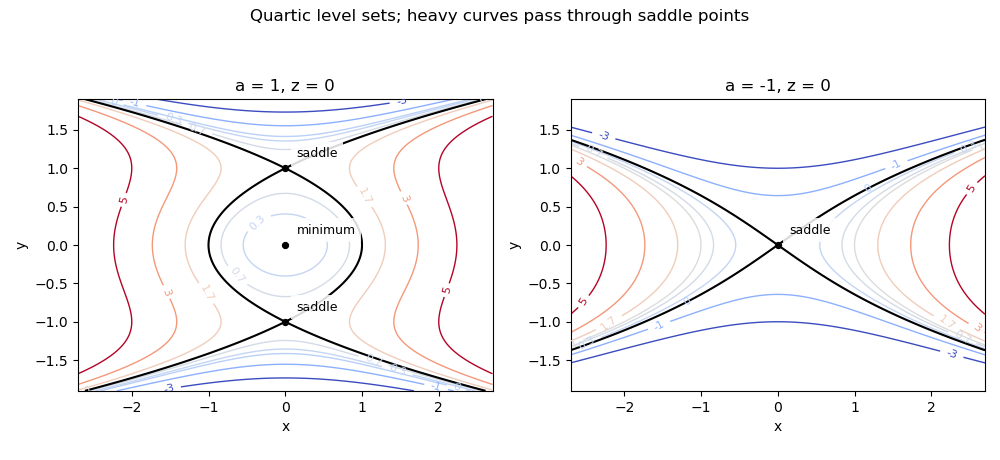
A stationary point requires $x=z=0$ and $y(a-y^2)=0$. The Hessian matrix is diagonal:For $a>0$, the origin has positive definite Hessian matrix, hence is a strict local minimum, with value zero. The two additional stationary points $(0,\pm \sqrt{a},0)$ have value $a^2$ and Hessian matrix $\mathrm{diag}(2,-8a,2)$; both are saddle points.

For $a<0$, the origin is the only stationary point and has an indefinite Hessian matrix, so it is a saddle point. For $a=0$, the Hessian matrix test is inconclusive, but $f(x,y,z)=x^2+z^2-y^4$ takes positive values along the $x$-axis and negative values along the $y$-axis arbitrarily near zero. Thus the origin is a degenerate saddle point. There are no local maxima in any case: varying $x$ or $z$ away from a stationary point increases $f$.

In the $(x,y)$-plane take $z=0$; holding another fixed $z$ merely shifts all contour labels by $z^2$. The level sets satisfyFor $a=1$, the origin is a local minimum and $(0,\pm 1)$ are saddle points of a scalar function at contour value $1$. For $0<c<1$, a closed contour around the origin is accompanied by unbounded outer components. At $c=1$ the contour satisfies $x=\pm (y^2-1)$ and crosses at the two saddle points of a scalar function. For $c>1$, two unbounded components remain; negative contours have only outer components.

For $a=-1$, the origin is a saddle point of a scalar function, and the zero contour is $x=\pm y\sqrt{y^2+2}$, with tangent lines $x=\pm \sqrt{2}y$. Positive contours form two components extending on opposite sides of the $y$-axis; negative contours form upper and lower components. These level sets are illustrated below.

The Wronskian isOn an interval where $p,q$ are continuous, the solutions are linearly independent exactly when $W(x_0)\ne 0$ at one point, equivalently when the Wronskian is nonzero throughout the interval. Differentiation and the homogeneous linear differential equation giveHence Abel identity reads $W(x)=W(x_0)\exp (-{\int }_{x_0}^{x}p(s)ds)$. If $W(x_0)=0$, the two initial-data vectors are dependent; the uniqueness theorem for ordinary differential equations then makes the corresponding linear combination identically zero. This proves the converse as well as the necessity.

Direct calculation givesWhere $1+\cos x\ne 0$, Abel identity gives $p=-W^{\prime }/W=\sin x/(1+\cos x)$, and substitution of either solution gives $q=1/(1+\cos x)$. ThusThese coefficients have singularities at odd multiples of $\pi$. This does not contradict the Wronskian criterion: its continuous-coefficient interval hypothesis fails at those points.

On $0\le x<\pi$, the initial conditions uniquely select $y=\sin x$. The normalized differential equation is not defined on the whole interval $0\le x<\infty$, so the usual global uniqueness theorem for ordinary differential equations cannot give the global initial-value assertion as posed. No choice of finite coefficients at $\pi$ can repair the normalized equation while retaining both displayed solutions: at that point $1+\cos x$ and its first derivative vanish, but its second derivative equals one.

The continuation through a zero of the leading ODE coefficient is a different problem: consider the multiplied, degenerate equationFor this different equation, a globally $C^2$ solution with the given initial data is uniquely $\sin x$. On each regular interval every solution is $A_j(1+\cos x)+B_j\sin x$; continuity of $y^{\prime }$ and $y^{\prime \prime }$ at an odd multiple of $\pi$ forces both constants to agree across it. If only $C^1$ piecewise solutions away from the singular points are required, the $A_j$ may change and uniqueness fails. Thus the coefficient singularity and the intended solution regularity must be distinguished.

Both functions satisfy the constant-coefficient homogeneous linear differential equationIts characteristic polynomial is $\lambda ({\lambda }^2+1)$, so the general real solution is $y=A+B\cos x+C\sin x$. The three initial conditions give $A+B=0$, $C=1$, and $-B=0$, henceHere the equation has continuous coefficients and nonzero highest-derivative coefficient everywhere. The uniqueness theorem for ordinary differential equations, applied to its three-component first-order system, gives a unique solution on the entire half-line.

Rewrite the integrand as $\sqrt{1-t{\cos }^2\theta }$. The binomial series, uniformly valid in $\theta$ for $|t|$ bounded below one, givesThe integrals of $1,{\cos }^2\theta ,{\cos }^4\theta$ over a full period are respectively $2\pi ,\pi ,3\pi /4$. Termwise integration therefore yields the ellipse perimeter expansion near a circle

With $t=1-x^2$ the chain rule gives $y^{\prime }=-2x{u}^{\prime }$ and $y^{\prime \prime }=-2u^{\prime }+4x^2{u}^{\prime \prime }$. Substitution, initially for $x>0$, givesThe transformed coefficients are $P(t)=1/t$ and $Q(t)=1/[4t(1-t)]$. At $t=0$, both $tP$ and $t^{2}Q$ are analytic; at $t=1$, both $(t-1)P$ and $(t-1{)}^{2}Q$ are analytic. Each point is singular because a normalized coefficient has a pole, but satisfies the regular singular point criterion for a second-order equation. Thus both points are regular singular points.

For a Frobenius method substitution $u=t^{\rho }{\sum }_{n\ge 0}{a}_n{t}^n$, the lowest power gives the indicial equationThe repeated indicial root is zero. Setting $\rho =0$ and equating the coefficient of $t^n$ givesConsequently the analytic power-series solution of a differential equation isTaking $a_0=2\pi$ reproduces the ellipse perimeter expansion.

For a second independent solution, normalize $u_1(0)=1$. Reduction of order and $P=1/t$ giveSince $u_1(s{)}^{-2}=1+O(s)$, this has the Logarithmic Frobenius solution formThe logarithm is $\log |t|$ on the real negative side, or a chosen complex logarithm on a slit complex neighborhood. Its nonzero logarithmic coefficient establishes independence. The physical perimeter is finite at $t=0$, so it selects the analytic branch rather than this logarithmic one.

By the definition of conditional probability,Since the $B_j$ form a disjoint partition of the sample space, the law of total probability gives $\mathbb{P}(A)={\sum }_j\mathbb{P}(A\mid B_j)\mathbb{P}(B_j)$. Substitution proves Bayes' theorem in the required form:The hypotheses make the denominator positive and each conditioning probability well defined.

Let $N$ denote the mattress count and $U$ the event of undisturbed sleep. Use the intended model in which the presence of the pea is independent of $N$, with probability $1/2$, and without a pea sleep is undisturbed. Conditioning on $N$ givesThe law of total probability and the equal prior probabilities giveBy Bayes' theorem, the posterior probabilities of $N=6,7,8$ given $U$ are respectively $5/18,6/18,7/18$. Therefore the conditional expectation isUndisturbed sleep shifts the posterior toward larger mattress counts because those counts make the observation more likely.

For any nonnegative random variable $X$ with finite expectation and any $a>0$, Markov's inequality statesIndeed $X\ge a{1}_{\{X\ge a\}}$, and taking expectations proves the bound. Nonnegativity is essential.

Each waiting time has the geometric distribution on $1,2,\dots$ with success probability $1/2$: a wait of length $n$ consists of $n-1$ failures followed by the prescribed success, so its probability is $2^{-n}$. HenceDisjoint successive blocks of independent tosses give independent waiting times. More explicitly, any specified list of block lengths determines exactly one allowed sequence of heads and tails and has probability $2^{-{\sum }_j(h_j+t_j)}$, the product of the individual block probabilities.

There are $2r$ waiting times. Multiplication of their probability generating functions and addition of their expectations giveTo recover its probability mass function, expand by the negative binomial series:The coefficient of $s^n$ is thereforeand it is zero below $2r$. Equivalently there are $\left(\genfrac{}{}{0ex}{}{n-1}{2r-1}\right)$ compositions of $n$ into $2r$ positive block lengths, each with probability $2^{-n}$. This is the negative binomial distribution for a sum of geometric waiting times, even though the desired outcome alternates between blocks.

For $r=1$,Since $\mathbb{E}{Y}_1=4$, Markov's inequality gives $\mathbb{P}(Y_1\ge 5)\le 4/5$, and indeed $5/16<4/5$.

Let $h_k$ be the hitting probability of the right endpoint before the left endpoint, starting at $k$. A surviving vase corresponds to that right-endpoint event. Conditioning on the first step of the simple symmetric random walk givesThe Markov property makes the remaining probability depend only on the position after that step. These absorbing endpoint values distinguish the event of interest from its complement.

Let $m_k$ be the expected remaining hitting time of either endpoint, measured in minutes. The first step consumes one minute, after which first-step analysis givesThe expectation is finite: from any interior state, a block of twenty leftward steps guarantees absorption and has probability $2^{-20}$. Thus the survival probability over successive twenty-step blocks has a geometric upper bound. This justifies using finite expectations in the recurrence.

The homogeneous linear recurrence relation has characteristic polynomial $(\lambda -1{)}^2$, hence general solution $h_k=A+Bk$. For the expected-time recurrence, rearrangement gives $m_{k+1}-2m_k+m_{k-1}=-2$, for which $-k^2$ is a particular solution. ThusImposing the absorbing boundary conditions from the preceding parts gives the gambler's ruin formulas

The initial position is $k=17$. Applying the gambler's ruin hitting probability and mean hitting time givesFor comparison, the original central starting position $k=10$ would give probability $1/2$ and mean time $100$ minutes.

Now the event is to hit $20$ before $1$, starting at $3$. Up to the first of those two hitting times, translate the interval by one unit; its endpoints become $0,19$ and the starting point becomes $2$. The gambler's ruin hitting probability is thereforeStopping at $1$ is essential: using the original absorbing endpoint $0$ would answer a different event.

Normalization of the probability density function givesThe first two moments areConsequentlyThe cumulative distribution function is $F(\varphi )=\varphi /\pi -{\varphi }^2/(4{\pi }^2)=1-(1-\varphi /(2\pi ){)}^2$ on $[0,2\pi ]$. For $U$ with the uniform distribution on $(0,1)$, inverse transform sampling therefore usesThe inverse lies in the required interval and satisfies $F(\Phi )=U$.

Conditional on $\Phi =\varphi$, the uniform distribution of the sector's centre angle gives a range of possible centre bearings of length $\varphi$ that hit a specified house. Independence of the two angles therefore gives the conditional probability $\varphi /(2\pi )$. By the law of total expectation,

For coverage of antipodal points by a randomly oriented sector, the house bearings differ by $\pi$. For $\varphi <\pi$, no single sector can cover both. For $\varphi \ge \pi$, the two allowable arcs of centre bearings overlap in two components, each of length $\varphi -\pi$. Thus the conditional probability of a double hit is $(\varphi -\pi )/\pi$, not $(\varphi -\pi )/(2\pi )$. Averaging against the probability density function givesPut $v=\varphi -\pi$ to obtain $\frac{1}{2{\pi }^3}{\int }_0^{\pi }v(\pi -v)dv$. Therefore

The event that $H_1$ is hit but $H_2$ is not has probability $1/3-1/12=1/4$. Dividing by the probability $1/3$ that $H_1$ is covered, using the definition of conditional probability, givesThis conditioning concerns angular coverage of a sector; the two house-hit events are not independent.