Past exam of the mathematics course of the University of Cambridge / 2013 / ib / Paper 1

The adjugate matrix is the transpose of the cofactor matrix: $\mathrm{adj}(A{)}_{ij}=(-1{)}^{i+j}\det A_{\hat{j},\hat{i}}$. Cofactor expansion gives the adjugate identityFor an invertible matrix this yields $A^{-1}=\mathrm{adj}(A)/\det A$. Integer entries of $A$ imply integer cofactors, so $\det A=\pm 1$ makes its inverse integral. Conversely, if $A$ and $A^{-1}$ both have integer entries, their determinants are integers and $(\det A)(\det A^{-1})=1$. The only integer units are $\pm 1$. Hence an invertible integer matrix has an integer inverse exactly when it is a unimodular matrix, with determinant $\pm 1$. Invertibility is implicit whenever $A^{-1}$ is used.

The zeroes of $\cosh z$ occur at $z=i\pi (n+\frac{1}{2})$, $n\in \mathbb{Z}$. They are simple because $\sinh z\ne 0$ there. Squaring the denominator therefore givesThere are no other finite singularities; this follows from the local zero-order criterion for a pole.

For $z\ne 0$, the denominator zeroes are $z_n=1/[\pi (n+\frac{1}{2})]$. Its derivative is $\sin (1/z)/z^2$, nonzero at each such point. ThusThese poles accumulate at zero. Consequently zero is a non-isolated singularity, as described by reciprocal cosine with accumulating poles. It is not an isolated essential singularity: no punctured disc about zero is a domain of holomorphy for this reciprocal function. Although $\cos (1/z)$ itself has an essential singularity at zero, taking its reciprocal introduces this accumulation of poles.

On the stated branch of the principal complex logarithm, the only denominator zero is $z=1$, and $\log z=(z-1)+O((z-1{)}^2)$. ThereforeZero is a logarithmic branch point, not a removable isolated singularity, even though $1/\log z$ tends to zero as $z\to 0$ within the cut plane. Continuation around zero changes $\log z$ by $2\pi i$. The nonpositive real axis is the chosen branch cut; its nonzero points are not intrinsically branch points and admit local analytic continuation. There are no other finite singularities inside the specified branch domain.

At $z=1$, numerator and denominator both have simple zeroes. Their derivatives give the removable valueAt each positive integer $n\ge 2$, the numerator is nonzero and the denominator has a simple zero, so these are simple poles. At zero the expansion on the principal sheet iswhich contains a fractional power. Thus zero is a branch point with pole-like leading growth, not an ordinary isolated pole. The negative real axis is the chosen branch cut. On local continuations across its nonzero points, negative integers also give simple poles because the continued square root is $\pm i\sqrt{|n|}$, never one. They lie outside the open principal branch domain; noninteger negative points are merely cut points, not intrinsic singularities.

Use the upper-half-plane model of the hyperbolic plane, whose geodesics are vertical lines and semicircles perpendicular to the real boundary. Hyperbolic and Euclidean angles agree. An isometry takes one of the ultraparallel hyperbolic lines to the imaginary axis. The other then has two finite endpoints on the same side; reflecting if necessary, write them as $0<a<b$. Its Euclidean centre and radius are $c=(a+b)/2$ and $r=(b-a)/2$.

A geodesic perpendicular to the imaginary axis must be a semicircle centred at zero, of some radius $q$. Two intersecting Euclidean circles meet orthogonally exactly when their squared centre distance equals the sum of their squared radii. Orthogonality to the second line therefore requiresSince $a<\sqrt{ab}<b$, the two semicircles intersect at one point in the upper half-plane. This constructs the common perpendicular of ultraparallel hyperbolic lines and proves uniqueness, because its radius is forced.

For the three-line continuation, the three common perpendiculars can be pairwise disjoint, but need not be. Explicit configurations of three ultraparallel lines make both claims transparent. For the positive example, take the three semicircles of radius $1/2$ centred at $-5/2,0,5/2$. Their endpoint intervals are disjoint. Their common perpendiculars are the semicircles with centres $-5/4,5/4,0$ and radii $\sqrt{21}/4,\sqrt{21}/4,\sqrt{6}$, respectively. The two smaller semicircles are disjoint because $2(\sqrt{21}/4)<5/2$; each is nested inside the largest because $5/4+\sqrt{21}/4<\sqrt{6}$. Hence their full geodesics are disjoint. For the negative example, take three concentric semicircles of radii $1,2,3$. They are pairwise ultraparallel, but every common perpendicular is the imaginary axis, so the perpendiculars coincide.

A convex function satisfies $g(tx+(1-t)y)\le tg(x)+(1-t)g(y)$ for all $x,y$ in its domain and $0\le t\le 1$. If the second derivative exists on an interval, this is equivalent to $g^{\prime \prime }\ge 0$ there. The equivalence follows from the nondecreasing first derivative, or from the supporting-line inequalities obtained by integration. HereThus it is a strictly convex function, and in particular convex.

For the Legendre transform, maximize $px-f(x)$ over $x>0$. Its derivative is $p-1-\log x$, and strict concavity makes the stationary point $x=e^{p-1}$ the unique maximizer. Substitution gives the convex conjugate of x log xThe range of $f^{\prime }$ is all of $\mathbb{R}$, so all real dual arguments have this finite value. Every point of the original graph is supported by its tangent of slope $f^{\prime }(x)$; the conjugate supremum therefore recovers $f$ from these supporting lines. Equivalently, the inverse derivative relation for this strictly convex differentiable Legendre transform gives $f^{\ast \ast }=f$ on $x>0$. If an extended-real function on all of $\mathbb{R}$ is wanted, its closed convex extension has value zero at $x=0$ and infinity for $x<0$; biconjugation includes that endpoint closure.

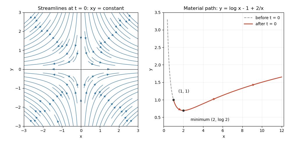
The divergence is ${\partial }_x{u}_x+{\partial }_y{u}_y=1-1=0$, while the scalar vorticity is ${\partial }_x{u}_y-{\partial }_y{u}_x=0$. The flow is therefore incompressible flow and irrotational flow. Integrating the streamfunction equations givesThe time dependence must be retained: no time-independent function $\psi (x,y)$ represents this unsteady field for every $t$. At $t=0$ the streamlines are $xy=\mathrm{constant}$, with the coordinate axes as separatrices. Their arrows point towards increasing $|x|$ and decreasing $|y|$, as shown below.

A pathline solves the material ODEs, givingFor $x_0\ne 0$, elimination of time yieldsIf $x_0=0$, the pathline stays on the $y$ axis and the parametric expression remains valid; it cannot in general be written as a single-valued $y=f(x)$ along that vertical trajectory. For $x_0=y_0=1$, the path is $y=\log x-1+2/x$: it initially descends, reaches its minimum $(2,\log 2)$, then rises. Unlike a frozen streamline, it records the time-varying flow.

For two-node Gaussian quadrature with linear weight, the monic node polynomial $q(x)=x^2-sx+p$ must be orthogonal to $1$ and $x$ for weight $x$. Indeed, exactness through degree three makes the quadrature of $q$ and $xq$ vanish at its nodes. The moment equations areso $s=6/5$ and $p=3/10$. Thus the Gaussian quadrature nodes, labelled in increasing order, areIntegrating the linear Lagrange interpolation cardinal functions gives the weightsThey are positive, sum to $1/2$, and reproduce the first moment $1/3$. Any cubic polynomial has remainder of degree at most one after division by $q$; orthogonality annihilates the other part both in the integral and at the nodes. This proves degree-three exactness, not merely the two moment conditions for the weights.

Let $M={\min }_i{x}_i$ and $S={\sum }_i(x_i-M)$. On the likelihood support $0<\mu \le M$, the log likelihood is $n\log \lambda -\lambda {\sum }_i(x_i-\mu )$. For fixed $\lambda$ it increases with $\mu$, so $\hat{\mu }=M$. Maximizing in $\lambda$ then gives the shifted exponential maximum likelihood estimatesThese finite estimates exist almost surely for $n\ge 2$. For one observation, or an all-equal sample, the likelihood is unbounded as $\lambda \to \infty$.

The minimum has $M-\mu \sim \mathrm{Exp}(n\lambda )$, so $E\hat{\mu }=\mu +1/(n\lambda )$: its bias is positive. By exponential memorylessness, $S\sim \mathrm{Gamma}(n-1,\text{rate }\lambda )$. For $n>2$, integration of the gamma density gives $E(1/S)=\lambda /(n-2)$, and henceAt $n=2$ this inverse moment is infinite, so a finite bias does not exist. Finally $E\overline{X}=\mu +1/\lambda =\beta$, so $\hat{\beta }$ is unbiased. The positivity assertions are therefore subject to the sample-size qualifications above.

In a zero-sum game with the row player maximizing, a sufficient saddle certificate is that $p,q$ are probability vectors andEvery row mixture then gains at most $v$ against $q$, and every column mixture concedes at least $v$ against $p$. Their pairing must equal $v$, proving optimality.

For the cost-weighted finite search game, order Colin's six columns as $123,132,213,231,312,321$ and Rowena's rows as $1,2,3$. The payoff matrix isUnder the proposed search mixture, an alternative location $i$ precedes the hiding location $j$ with probability $(c_i+c_k/2)/c$, where $k$ is the third location. The expected cost conditional on hiding at $j$ is consequentlyIt is independent of $j$, giving the upper bound $\mathrm{value}\le v$.

Choose $p_i=c_i/c$. Against any order $i,j,k$, its expected cost isThis gives the matching lower bound. ThusBoth strategies equalize the opponent's pure actions, giving the stated saddle certificate.

The external direct sum of vector spaces consists of pairs $(v_1,v_2)$ with componentwise operations. For subspaces of one ambient space, the sum of vector subspaces is $V_1+V_2=\{v_1+v_2:v_i\in V_i\}$. The addition map from the external direct sum onto this subspace is surjective, with kernel $\{(w,-w):w\in V_1\cap V_2\}$. This kernel is isomorphic to the intersection. The rank-nullity theorem, together with $\dim (V_1\oplus V_2)=\dim V_1+\dim V_2$, proves the dimension formula for a sum of subspaces.

For the supplied bases, solving for annihilating linear forms givesEach basis has rank three, so these hyperplanes are the whole subspaces. The two independent equations make the intersection two-dimensional. Imposing the requested zero components yieldsBoth satisfy the two equations and are independent, since their first components differ while $v_1\ne 0$. Hence they form the required basis.

The coordinate axes are exactly the simultaneous eigenspaces of all invertible diagonal matrices in $T$. A matrix normalizing $T$ must permute these common eigenspaces: if $tv=\chi (t)v$, then $t(gv)=g(g^{-1}tg)v$ is again a scalar multiple of $gv$. Thus a normalizer element has exactly one nonzero entry in each row and column, a monomial matrix. In dimension two it is either diagonal or diagonal times $J=\left(\begin{array}{cc}0& 1\\ 1& 0\end{array}\right)$. Conversely $J$ swaps the diagonal entries and normalizes $T$. ThereforeThis is the normalizer of a diagonal subgroup of GL2; the quotient records the permutation of the two axes.

For a prime $p>2$, a diagonal matrix with two distinct nonzero eigenvalues exists. The same common-eigenspace argument makes the normalizer of a diagonal subgroup of GL2 precisely the monomial matrices. There are $(p-1{)}^2$ choices of nonzero entries for each of two permutation patterns, givingAt $p=2$, however, the invertible diagonal subgroup is trivial. Every invertible matrix normalizes it, soThe first factor chooses a nonzero first column and the second chooses a column outside its one-dimensional span. The exceptional answer is necessary because the printed question permits every prime.

For uniform convergence to $k$ on $A$, for every $\eta >0$ there is $N$ such that $|k_n(x)-k(x)|<\eta$ for all $n\ge N$ and all $x\in A$. The bound $|\sin (nx)/\sqrt{n}|\le 1/\sqrt{n}$ proves uniform convergence to zero, whereas its derivative is $\sqrt{n}\cos (nx)$. On an interval containing zero these derivatives diverge at zero, so they cannot converge uniformly. This supplies a counterexample to differentiating a uniformly convergent sequence without additional hypotheses.

For uniform derivative convergence with an anchored value, put $g=\lim k_n^{\prime }$ and $a=\lim k_n(x_0)$. A uniform limit of continuous functions is continuous. The fundamental theorem of calculus givesThus $k_n(x)\to k(x)=a+{\int }_{x_0}^{x}g(t)dt$, with error bounded byThis is uniform on bounded subintervals, and on all of $A$ if it is bounded. The fundamental theorem of calculus now gives $k^{\prime }=g$, so $k$ is continuously differentiable. For an unbounded $A$, no global uniform convergence of $k_n$ follows merely from the displayed hypotheses, but local uniform convergence and the claimed differentiability do.

For the series, use partial sums and differentiate their individual terms:For $|x|\le 1$, their absolute values are at most $2n/(n^3+1)$, a summable bound. The Weierstrass M-test makes the derivative series uniformly convergent, while every partial sum is zero at $x=0$. The anchored-value result therefore proves continuous differentiability on $(-1,1)$, with derivative equal to the displayed termwise derivative series.

The sphere is the inverse image of $\{1\}$ under the continuous map $u\mapsto \Vert u{\Vert }^2$, so it is closed in ${\mathbb{R}}^3$. It is bounded. The Heine-Borel theorem therefore makes it compact. Every metric space is Hausdorff: distinct points have disjoint open balls of radii smaller than half their distance. The Euclidean subspace metric supplies that property here. Hence $S^2$ is compact and Hausdorff.

The quotient map $q:S^2\to X$ is continuous and surjective by the quotient topology, so $X$ is compact as a continuous image of a compact space. To prove the Hausdorff property explicitly, let $[u]\ne [v]$ and set $d=\min (\Vert u-v\Vert ,\Vert u+v\Vert )>0$. Choose $r<d/3$. The saturated open setsare disjoint by the triangle inequality. Each contains both antipodes of every one of its points, so $q^{-1}(qU)=U$ and similarly for $V$. Consequently $qU,qV$ are disjoint open quotient neighborhoods separating the classes. Thus the quotient is compact and Hausdorff. It is the real projective plane; equivalently the metric on the antipodal sphere quotient is $d_X([u],[v])=\min (\Vert u-v\Vert ,\Vert u+v\Vert )$ and induces this topology.

Write $p(z)=c{\prod }_{j=1}^{2m}(z-a_j)$, including root multiplicities. For $|z|>R$ the convergent logarithm series for every factor $1-a_j/z$ definesChoosing either square root of the nonzero leading coefficient gives the holomorphic square root outside all polynomial rootsIts square is $p$. The even degree makes $z^m$ single-valued, avoiding the winding obstruction that an odd degree would create on the exterior annulus.

For the branch behaving as $z^2$ at infinity, the Laurent series isIt converges uniformly on the circle of radius two. Only the coefficient of $z^{-1}$ contributes to its anticlockwise integral, sofor this branch, and $+\pi i$ for the other. These are the two allowed answers.

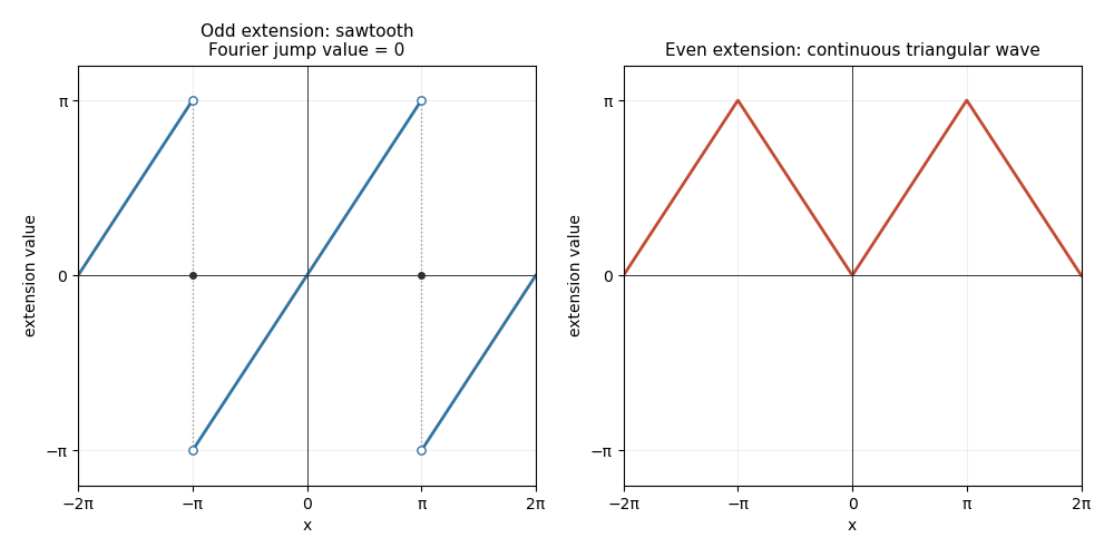
Integration by parts gives the Fourier sine series coefficientsHenceThe odd periodic extension is a sawtooth, equal to $x$ on $(-\pi ,\pi )$ and repeated every $2\pi$; its jumps at odd multiples of $\pi$ have midpoint value zero in the Fourier series. In particular the sine series equals zero, rather than the specified endpoint value $\pi$, at $x=\pi$. The even periodic extension is the continuous triangular wave equal to $|x|$ on $[-\pi ,\pi ]$. Their sketches are below.

The Parseval identity for a Hilbertian basis for this sine expansion gives

Use the drift-removing substitution for a Dirichlet Sturm-Liouville problem, $y=e^{-x}v$. Direct differentiation gives $\mathcal{L}y=e^{-x}(-v^{\prime \prime }+v)$. The homogeneous boundary conditions become $v(0)=v(\pi )=0$, so the eigenvalues and eigenfunctions areThe self-adjoint weighted form isThus the weight and leading coefficient are both $e^{2x}$. The orthogonality of Sturm-Liouville eigenfunctions readsAfter multiplying the forcing equation by $e^x$, it becomes $-v^{\prime \prime }+v=x$. Expanding $x$ in the sine series of part (i) and dividing by $n^2+1$ givesEvery term satisfies the endpoint conditions. As a check, solving the transformed ODE directly gives $v=x-\pi \sinh x/\sinh \pi$, which has the same coefficients and forcing.

Using the momentum operator $\hat{p}=-i\hslash d/dx$ and its commutator with multiplication by $A$, expansion of the factorized quantum Hamiltonian givesThe first-order zero-mode equation integrates toFor $A=x^n$, its exponent is $-s{x}^{n+1}/[\hslash (n+1)]$. It decays at both ends exactly when $n+1$ is even. If $n$ is even it grows at negative infinity. Thus a nonzero square-integrable zero mode exists exactly for odd $n$.

For $n=1$ the Gaussian zero mode is $\chi =(s/(\pi \hslash ){)}^{1/4}{e}^{-s{x}^2/(2\hslash )}$. More generally, on normalized states with finite second moments and the usual integration-by-parts boundary conditions, $\hat{H}=Q^{†}Q/(2m)$ is nonnegative. With zero means this implies, for every $s>0$,Minimizing the quadratic in $s$ at $s=\hslash /[2(\Delta x{)}^2]$ yieldsThe Gaussian mode attains equality. The argument concerns the same state for the whole positive family of factorized operators, which permits the minimization.

The Drude model treats carriers as classical independent particles, accelerated between collisions by the electric force. Collisions occur at constant rate ${\tau }^{-1}$ and randomize the directed velocity to zero mean; the ions are an effectively stationary background. Over a short time $dt$, directed velocity gains $(e/m)\mathbf{E}dt$ while the fraction $dt/\tau$ that collides loses its mean directed motion. ThereforeHere $e$ is the signed carrier charge. For the stated complex harmonic convention,The conductivity is positive in its dissipative real part regardless of the sign of $e$.

For zero charge density, Gauss's law makes the electric amplitude transverse. Faraday's and Ampère-Maxwell's laws, with displacement current retained, giveSubstitution of $e^{i\mathbf{k}\cdot \mathbf{x}-i\omega t}$ yieldsFor propagation in a fixed direction, $k$ is the possibly complex scalar wave number; equivalently the spatial equation uses $\mathbf{k}\cdot \mathbf{k}$, without complex conjugation. The printed real-vector notation $|\mathbf{k}|$ must be analytically continued in an absorbing or evanescent medium.

In the high-frequency Drude plasma cutoff regime, $\omega \tau \gg 1$ gives ${ϵ}_r\simeq 1-{\omega }_p^2/{\omega }^2$. Below the plasma frequency, the physical decaying branch isFinite collisions add a small phase component while maintaining positive attenuation. Very near the threshold one should retain the full complex permittivity rather than the purely imaginary approximation.

For inviscid flow with a conservative body-force potential $\Phi$, the Euler momentum equation and the identity $(\mathbf{u}\cdot \nabla )\mathbf{u}=\nabla (|\mathbf{u}{|}^2/2)-\mathbf{u}\times (\nabla \times \mathbf{u})$ apply. In an irrotational region write $\mathbf{u}=\nabla \varphi$. For constant density they giveThis is the Unsteady Bernoulli equation; its constant is spatially uniform, with time-dependent gauge absorbed into $\varphi$ if desired.

For the intended linearly elastic balloon discharge model, take an initially stationary, inviscid plug of water in the constant-area tube. Put $B=\pi a^2$ and $p_{\mathrm{in}}-p_{\mathrm{atm}}=KV$ with $K>0$. At the two tube ends the speeds are equal, so their kinetic terms cancel in the Bernoulli difference. Since $\varphi (L)-\varphi (0)=Lu$, this givesHence $\ddot{V}+{\Omega }^{2}V=0$, where ${\Omega }^2=KB/(\rho L)$. With $V(0)=V_0$ and $u(0)=0$,ThusAcceleration stays positive until emptying, so the maximum speed is reached at that instant. The time is independent of initial volume, while the maximum speed is not.

The initial-rest condition is implicit in the claimed volume independence, rather than specified in the text. For an independently prescribed positive initial speed $u_0$, the first zero instead occurs at ${\Omega }^{-1}\arctan [\Omega V_0/(B{u}_0)]$. The calculation also takes the given balloon pressure as the pressure directly at the tube entrance; a reservoir-to-exit kinetic-head or entrance-loss model would add other terms and is not this equal-speed tube model.

For a full-column-rank matrix, a thin QR decomposition has $A=Q_{1}R$, where $Q_1^T{Q}_1=I_n$ and $R$ is nonsingular upper triangular. Extend $Q_1$ to an orthogonal matrix $Q=(Q_1,Q_2)$. Orthogonality givesThus the unique least-squares solution satisfies $R{x}^{\ast }=Q_1^{T}b$, with residual norm $\Vert Q_2^{T}b\Vert$. In a rank-deficient problem $R$ is singular and uniqueness needs separate treatment.

A Givens rotation is the identity except for the rows/columns $p,q$, whose block is $\left(\begin{array}{cc}c& s\\ -s& c\end{array}\right)$ with $c^2+s^2=1$. Its transpose times itself has that block equal to the identity, so it is orthogonal. Choose $c=4/5,s=3/5$ in rows two and three. ThenBack substitution in the first three rows givesThe fourth row of the rotated residual is the unavoidable value $-2$, while the other three rows vanish. Thus this rotation also directly exhibits the least-squares optimality.

Let $H=X(X^{T}X{)}^{-1}{X}^T$ be the orthogonal projection onto the design column space. Linear transformations of the Gaussian errors giveThe residual distribution is a singular multivariate normal supported on the orthogonal complement of that column space. Their cross-covariance is ${\sigma }^2(X^{T}X{)}^{-1}{X}^T(I-H)=0$. Joint normality even makes the two vectors independent.

Order the observations as $11,12,21,22$. The two normal linear models have design matricesRemoving each row mean leaves the information for the common slope equal to the sum of within-row squared fertilizer deviations. These sums are $1$ and $4$, respectively. ThereforeThe second design estimates the slope four times as precisely in variance terms.

The observed data in the second design are fitted exactly by $\hat{\theta }=(100,300,100{)}^T$. With $a=(2,2,0{)}^T$, the no-fertilizer total forecast isThe future four independent errors contribute variance $4{\sigma }^2$. Parameter-estimation uncertainty contributes ${\sigma }^2{a}^T(X_{II}^T{X}_{II}{)}^{-1}a=13{\sigma }^2$, so the prediction-error variance is $17{\sigma }^2$, not merely the variance of the estimated mean. Normally, with $s^2=\Vert \widehat{ϵ}{\Vert }^2/(4-3)$, the prediction interval in a normal linear model isHere the printed data have zero residual and hence $s=0$. The formal plug-in interval collapses to $[800,800]$, exhibiting zero-residual degeneracy of regression prediction. Under the stated model with unknown positive variance, this exact fit is a probability-zero sample and the Studentized statistic is undefined at it; the collapsed expression is not evidence that future yield is certain. No positive-width numerical 95% interval can be obtained from these exact data by the usual residual-variance method without extra variance information or an explicit observation-rounding model.

First realize the chain as a random walk on a multigraph: put three parallel edges between $a,b$, two between $a,c$, and one between $b,c$. There are six edges and vertex degrees $5,4,3$. Choosing an incident edge uniformly gives exactly the stated transition probabilities. The stationary distribution of a graph random walk is the degree divided by twelve, $\pi =(5,4,3)/12$, and detailed balance follows because each edge multiplicity contributes the same flux in both directions.

For the first positive return time, Kac's lemma givesFor passage to $b$, put $h_a=k(a,b)$ and $h_c=k(c,b)$. The first-step equations are $h_a=1+(2/5)h_c$ and $h_c=1+(2/3)h_a$, since reaching $b$ stops the clock. ThusA multigraph is essential: a simple graph on three vertices cannot have six edges.

Let $T_i$ be the expected time to complete the specified directed transition, starting at $i$. This is a transition-completion time in a Markov chain, rather than merely a first visit to $c$. First-step decomposition givesThe missing $b\to c$ continuation in the middle equation represents successful completion, but its step is counted by the leading one. Substitution givesThus the requested expectation from $a$ is $128/11$ steps.

The chain is a reversible Markov chain, so detailed balance makes the stationary path probabilityA path contains an ordered occurrence of $a$ followed later by $b$ exactly when its reversal contains $b$ followed later by $a$. These occurrences need not be adjacent. Therefore $\mathrm{Pr}(\tau (a,b)\le m)=\mathrm{Pr}(\tau (b,a)\le m)$ for every $m$, and in particular the two finite expectations are equal. This is ordered-state visit times in a reversible chain.

To decompose the expectations, distinguish the entrance time $h(i,j)$, which allows time zero and has $h(j,j)=0$, from the positive return convention $k(j,j)$ in part (i). The Strong Markov property at the first visit to $a$ or $b$ givesEquating them yields the difference formula with $h$. Replacing $h$ by $k$ in the sum adds ${\pi }_{a}k(a,a)-{\pi }_{b}k(b,b)=1-1=0$, again by Kac's lemma. HenceFor a numerical consistency check, the other entrance times are $k(b,a)=15/11$ and $k(c,a)=16/11$, while $k(b,b)=3$. Both sides of the displayed identity equal $-6/11$.