In Cartesian coordinates, write and use the Levi-Civita symbol. The contraction of two Levi-Civita symbols givesHere the Kronecker delta selects the indicated indices, and continuous second partial derivatives allow their order to be interchanged. Identifying the gradient, divergence and componentwise Laplacian proves the curl of the curl identity:
Let be a bounded region with piecewise smooth closed boundary , let be its outward unit normal vector, and let be a continuously differentiable vector field on a neighbourhood of its closure. The divergence theorem statesHere is the positive volume measure, is the surface area measure, , and the right side is the total outward flux. All boundary components must be included, with their normals pointing away from .
Differentiate the position vector with respect to the three coordinates:Their pairwise dot products vanish. For example, . Thus these are orthogonal coordinates wherever the coordinate tangents are nonzero. Their scale factors of orthogonal coordinates areThe absolute Jacobian determinant is their product, givingThe ordered coordinate system is left handed: . The volume measure uses the absolute value. The axis and the focal circle contain coordinate degeneracies, as expected for oblate spheroidal coordinates. This is the hyperbolic parametrization of oblate spheroidal coordinates. The local TeX has an OCR substitution in the volume formula; the original PDF correctly prints .
Put . For , elimination of givesThese are oblate spheroids with equatorial radius and polar radius , flattened along the axis. At the limiting surface is the disk , .
For , elimination of instead givesThese are one-sheet hyperboloids of revolution, restricted to their upper half for and lower half for . The restriction matters because . At , the surface degenerates to the exterior equatorial plane , ; at it degenerates to the corresponding half of the axis.
Finally, fixed specifies a vertical half-plane through the axis, with horizontal direction . The two values and together give a full plane. These surfaces form the mutually orthogonal families of the hyperbolic parametrization of oblate spheroidal coordinates.
For a nondegenerate surface take , and abbreviate , . Close the upper oblate spheroid by its equatorial disk , obtaining a half-ellipsoid . The divergence isThe integral of vanishes by reflection symmetry. At height , the cross-section is a disk of radius . Using planar polar coordinates,ConsequentlyThe outward unit normal vector on is , so its flux is . Applying the divergence theorem to the closed surface and subtracting this disk contribution givesThis is a special case of polynomial flux through a half-ellipsoid. Including the closing disk is essential: the constant vertical component has zero divergence but nonzero flux through the open curved surface.
Seek a nonzero separated solution . Substitution into the heat equation and division by the product givesThe left side depends only on time, so set it to . Multiplication by then separates the angular dependence, with separation constant . The three ordinary differential equations areThe temporal solution is . With , the angular equation is the Legendre differential equation; regularity at both angular endpoints selects and , the Legendre polynomial. The radial equation has the Spherical Bessel functions and for . Regularity at , if imposed, excludes the singular second solution. For the radial powers are and . Without specified radial boundary conditions, no discrete set of is selected; is a convention for the temporal separation constant.
For spherical symmetry the angular mode is . Put . Direct differentiation givesso the radial heat equation in three dimensions becomes the ordinary one-dimensional heat equation . Since , the zero endpoint temperatures become .
Write . The two initial sine modes already satisfy these Dirichlet boundary conditions; their squared wave numbers are and . Each therefore evolves independently with its corresponding exponential decay. Dividing back by givesAt the initial profile is recovered, and each sine is zero at both endpoints. The first mode decays four times more slowly in its exponential rate than the second. This is the two-mode instance of the spherical-shell heat equation via radial rescaling; uniqueness follows, for example, by applying the heat equation energy identity to the difference of two solutions.
For a fixed source point , the Green function is defined bywhere is the Dirac delta distribution and the operator acts on . The corresponding solution isApplying under the integral gives by the defining delta identity, while the endpoint values vanish. With the stated continuous coefficients, one may define the normalized distributional equation ; this avoids multiplying a general distributional second derivative by a merely continuous coefficient.
Existence of this inverse Green function additionally requires that the homogeneous two-point boundary value problem have only the zero solution. The assumptions printed in the question alone do not ensure this: on has the nonzero zero-endpoint solution . At such resonance there are solvability conditions and no ordinary inverse kernel for arbitrary . The construction below is nonresonant.
Suppose the piecewise smooth Green function has jump . Its first distributional derivative then contains , and its second contains . In the normalized equation from part (a), the first-derivative term can supply a delta but no delta derivative. The right side has only a delta. Thus its delta-derivative coefficient must vanish:Equivalently, the two homogeneous branches must join continuously. This is the continuity part of the jump condition for a second-order Green function.
Now is continuous, so has no delta contribution. Integrate its normalized differential equation over . The bounded lower-order terms have integrals tending to zero, while the integral of is the difference of the two one-sided first derivatives. Hence the jump condition isThe denominator is evaluated at the source point; it is not a variable left over after taking the limits. The positivity or negativity of this jump follows the sign convention used for the leading coefficient of .
The homogeneous characteristic equation is , with roots . Choose the endpoint-adapted homogeneous solutionsso that and . Their Wronskian iswhich never vanishes. A continuous Green function with the required endpoints has the form , where and . Its derivative jump is . Because the leading coefficient is one, part (b) requires this to equal one. ThereforeIn particular, the branches are for and for . This is the Dirichlet Green function for a conjugated harmonic oscillator with interval length , drift parameter one and oscillator wave number one.
Insert the source into the Green-function representation and split the integral at its source discontinuity in derivative:Using , the answer isBoth endpoint values are zero. As a direct check, conjugating by sends to , and gives . Thus the differential equation and both boundary conditions are satisfied.
First take a Schwartz function, so that Fourier inversion and the exchange of integrals are justified. Inserting the inverse transform of the complex conjugate givesFor , approximate it by Schwartz functions in both norms. The identity just proved makes their transforms a Cauchy sequence in L2 space, while convergence in L1 space makes the transforms converge uniformly to the defining transform of . Thus the two transform limits agree, and passing to the norms proves the finite Parseval identity. This is the normalization of the Plancherel theorem appropriate to the paper.
There is a qualification to the printed hypothesis: absolute integrability alone does not guarantee a finite square integral. For instance on and zero elsewhere belongs to but not . For an function of this kind the transform is not in either, by L2 density from a square-integrable Fourier transform, so both sides are infinite if the identity is interpreted in that extended sense. The finite equality requires square integrability as well.
Use the trigonometric identity and express the cosine as a sum of two complex exponentials. The Fourier transform of each exponential is a shifted Dirac delta distribution:By linearity,The original function does not decay and is not absolutely integrable on the real line, so this answer is a tempered distribution, rather than an ordinary convergent Fourier integral. Its three lines represent the constant part and the two opposite spatial frequencies.
The input is even, so its Fourier transform is real and even. Decomposing the cosine into complex exponentials and integrating over its support givesCombining the fractions and using the angle addition formula yieldsThe apparent poles at are removable singularities; either the integral or the sine-quotient limit gives .
If , expansion of the denominator givesThe oscillatory envelope is therefore . At , , the endpoint values vanish and the first term cancels:This gives an envelope. At general the truncation creates jumps in the function; at these special values it leaves the function continuous but creates jumps in its first derivative. Each additional degree of endpoint smoothness gives another inverse power, as explained by Fourier decay from a derivative jump. The exact example is the Fourier transform of a truncated cosine; isolated zeros of its oscillatory factors do not change the envelope order.
The columns of are an orthonormal basis, since and the first two columns have zero dot product. Thus : it is an orthogonal matrix. Consequentlyand hence . This is the preservation of the Euclidean norm by a rotation matrix.
The direction is fixed, giving the eigenvalue one. The planar block has characteristic polynomialThus the full list of eigenvalues isThe last two are real precisely when , so all three are real exactly for . At even multiples of the matrix is the identity and every vector is fixed. At odd multiples it is a half-turn: the axial eigenvalue remains , while the whole perpendicular plane has eigenvalue .
For other angles, the only real eigenvector direction is the rotation axis; the perpendicular plane is rotated rather than preserving an individual real direction. Its complex eigenvectors can be taken as and for and , respectively. These represent the two complex conjugate planar eigenvalues.
With the same right-handed active rotation convention as , the direction is fixed, rotates towards , and towards . ThereforeIts columns give the images of the three Cartesian unit vectors, which also makes the signs of this rotation matrix explicit.
A product of orthogonal matrices is orthogonal. In fact,Thus Its determinant is also one, since each factor has determinant one, so it remains a proper rotation matrix.
Both factors and their product are real, so the Hermitian conjugate equals the transpose. Part (i) therefore givesHence A real orthogonal matrix is always a unitary matrix.
A real matrix is a Hermitian matrix exactly when it is a symmetric matrix. Since is orthogonal, this is equivalent to , or . A generic rotation does not satisfy this; for example , gives a nonsymmetric quarter-turn. Thus
The exceptions are the identity and half-turns, as characterized by real rotation matrices that are Hermitian. For this product, a half-turn occurs when either or is an odd multiple of ; the identity occurs when both are even multiples. For example, the half-turn condition follows from .
The Hermitian conjugate of a real matrix is its transpose, soTherefore It is also a real skew-symmetric matrix. It is Hermitian as well only in the exceptional case , precisely when is symmetric. This includes the identity and half-turn cases from part (d), so the zero-matrix overlap should not be excluded.
Applying the rightmost rotation matrix first givesEquality with requires , so in the specified range. Then and giveIn the reverse order, first fixes , so . Therefore . This explicitly demonstrates that rotations about different axes do not generally commute.
At the angles in part (f),Let the two diagonal matrices be and . Multiplication givesThe vector condition is exactly . For , the general form is thereforeEvery pair is attainable, for example with and . The transformation need not be orthogonal or invertible; the question asks only for diagonal rescalings with this one vector image. If and , no linear map can satisfy the condition. If , the entry is arbitrary as well.
Let be a Hermitian matrix and with . The scalar equals its own complex conjugate, becauseSince and the squared norm is positive, .
Now take and . The inner product satisfiesSubtracting gives . Thus distinct eigenvalues imply , proving orthogonality of the corresponding eigenvectors. Within a degenerate eigenspace, an orthonormal basis may be chosen, but arbitrary distinct vectors in that same eigenspace need not be orthogonal.
A complex square matrix is a unitary matrix if . Equivalently, it preserves the complex inner product and hence the norm. If with , thenDivision by the positive squared norm gives . Thus every eigenvalue lies on the unit circle.
All factors that are rational functions of commute. Taking the Hermitian conjugate reverses product order and givesThereforeso . This is a Cayley transform of a Hermitian matrix, with scale and the convention that an infinite real eigenvalue maps to one.
Applying it to each eigenvector yieldsThe eigenvectors are unchanged, and because numerator and denominator are complex conjugates. No equals one when . The scalar map is injective on real , so the eigenspaces, including any degeneracies, are preserved exactly.
Use and take the Hermitian conjugate in the reverse product order:The factorization gives , while . ConsequentlyThe last equality uses the fact that commutes with and its inverse. Thus is a Hermitian matrix. The exclusion of the eigenvalue one is essential to define the inverse. Spectrally, an eigenvalue is sent to , a real number. This is the inverse Cayley transform of a unitary matrix without eigenvalue one.
For a holomorphic function with , the chain rule givesWriting and equating real parts and imaginary parts,For , division by gives the Cauchy-Riemann equations in polar coordinates:The restriction reflects the coordinate singularity at the origin; the Cartesian equations have no such restriction.
Insert the specified real part into the polar Cauchy-Riemann equations. The first gives , and integration with respect to givesThe second equation then requires , so . The remaining imaginary additive constant is fixed by . ThusThe resulting polynomial is holomorphic at the origin too, consistently extending the calculation made in polar coordinates with .
Using the exponential form of the complex cosine, is equivalent to . Thus the zeros are exactlyAt each point , so the cosine has a simple zero. Cubing it givesThe order of a zero of a holomorphic function is therefore three at every zero. There are no finite singularities because this is an entire function.
To classify infinity, examine at . The identity shows that its Laurent series contains the nonzero negative-power coefficientsThere are infinitely many terms in the principal part, the criterion for an essential singularity. Therefore This is also the general characterization of a nonpolynomial entire function at infinity.
If , factor out and use the geometric series:ThusThe radius of convergence is the distance to the nearest singularity, the simple pole at . The case must be treated separately: the function is , has no Taylor series about zero and is already its own Laurent series on .
For , multiply the absolutely convergent Taylor series of the sine by the geometric series:The product is odd, so all even coefficients vanish. Collecting the coefficient of givesFor example, the first terms are . The denominator vanishes at , and the numerator is nonzero there, so these are genuine simple poles. Therefore is the radius of convergence.
After division by the leading coefficient, write , whereThe only finite singular points of a differential equation are . At zero, and are analytic. At , and are analytic. The regular singular point criterion for a second-order equation therefore makes both points regular.
If infinity is included, it is a regular singular point at infinity as well: and . Equivalently, with the transformed coefficients are and , which satisfy the same regular-singular criterion at .
For the Frobenius solution, differentiate term by term:The unshifted terms in the equation have coefficient . The extra factors of give the shifted contribution . Equating the coefficient of for gives the linear recurrence relationFactoring both coefficients is especially useful:The separate lowest-power equation is . Do not cancel when it vanishes: that is the possible undetermined coefficient at Frobenius resonance.
Because , the lowest-power equation from part (b) requires the indicial equationThe two candidate indicial roots are thereforeTheir difference is the integer one, so the smaller-root coefficient equation at needs examination rather than automatic division.
For the larger indicial root , the recurrence in part (b) becomesNo factor being cancelled is zero in this range, soThus the resulting Frobenius solution isThere is exactly one free parameter, , setting the overall scale. The analytic series factor has radius of convergence one. For a real-valued expression take ; a complex version requires a local square-root branch.
The Taylor series of the logarithm givesTherefore the closed form of the larger-root Frobenius solution isThe series derivation holds initially for ; the closed form extends as a real solution to all . To check it without series, put in the original equation. All undifferentiated terms cancel and the remaining expression is . Hence , and indeed solves it. Its logarithm is analytic near zero, so this is not a forced companion term at the Frobenius point.
At the smaller indicial root , the equation is : it leaves free. For , the valid recurrence isChoosing makes every later coefficient zero. The resulting terminating Frobenius series is thereforeSubstitution gives and ; the three terms in the equation sum to .
Termination is a permitted choice, not a condition forced on every smaller-root solution. Retaining the free adds the solution in part (e), so the general real solution on is . This is exactly the freedom explained by undetermined coefficient at Frobenius resonance. On either negative interval avoiding and , analogous real formulas use and .
For fixed endpoint values, a stationary differentiable path obeys the Euler-Lagrange equationIt follows by taking the first variation of the functional and integrating the term in by parts; vanishes at the endpoints.
If has no explicit dependence, the chain rule givesConsequentlyon an Euler-Lagrange equation solution. Thus the Beltrami identity supplies the first integralThe opposite sign is an equally valid convention. The conserved value can be zero for particular integrands or paths; absence of explicit alone does not guarantee a nonzero numerical value. The useful statement is that this expression is constant along an extremal.
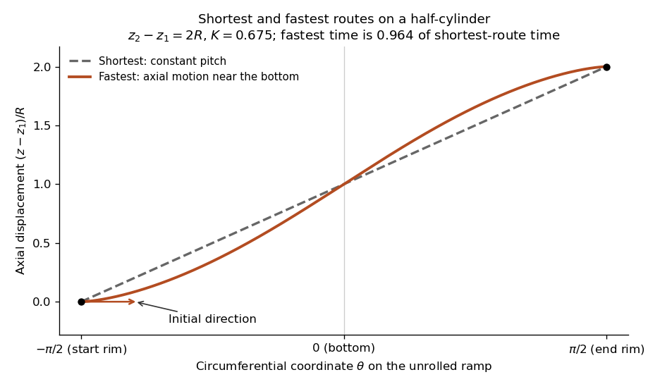
On the cylindrical surface , the line element is . For a single-valued path parametrized by increasing ,The integrand has no explicit , so its Euler-Lagrange equation gives the constant conjugate quantity . Its derivative with respect to is strictly positive, hence itself is constant. The two endpoints determineThis is a constant-pitch helix on the cylinder. To verify global minimality, unroll the cylinder with planar coordinates . The path becomes a straight line between points separated by and , so the triangle inequality for arc length givesThis is the standard description of geodesics on a circular cylinder.
The downward drop from the starting rim to angle is . With no dissipative forces, conservation of energy gives , so . Dividing the line element by this speed yieldsThe endpoint singularities are integrable for the minimizing path. The integrand is independent of ; its Euler-Lagrange equation gives a constant , after absorbing the overall prefactor:Solving for and taking the positive branch required by givesThe constant is fixed implicitly byThis integral is strictly increasing from zero to infinity as increases from zero to one, so every finite positive separation selects a unique . The time integrand has second derivative with respect to . Its supporting-line inequality, integrated between fixed endpoints with constant first derivative with respect to , proves this stationary path is the unique global minimum within the stated single-valued class.
As , . Therefore the skater should initially head directly down the curved ramp, perpendicular to the cylinder axis, and gain axial motion later. The path differs from the constant-pitch shortest route because extra distance is cheaper in time near the faster, lower part of the ramp. This is the brachistochrone on a horizontal half-cylinder.

Articles were limited to the first 100 out of 111 total.
Articles by others on the same topic
There are currently no matching articles.