Take to mean that the mirror recedes along the incident plane electromagnetic wave. Put , with . The moving-mirror Doppler shift can be obtained directly by matching wave phase on the moving surface. Write the incident wave phase as and the reflected wave phase as , where and are positive wavenumbers. At the mirror, , the two phases must have the same time dependence; their constant offset incorporates the reflection phase shift. ThusConsequently the observed reflected angular frequency and ordinary frequency areThis is a redshift for a receding mirror and a blueshift for an approaching mirror. At small velocity, .
Equivalently, the relativistic Doppler effect gives in the mirror rest inertial frame. Reflection there reverses propagation and preserves frequency. Transforming the backward-going reflected wave to the laboratory gives another factor , so . A single Doppler factor would miss the effect of the return path.
Use a transparent reciprocal wave plate at its design wavelength. For the return calculation, assume a mirror at normal incidence with the same reflection coefficient for both transverse components; this is the usual ideal double-pass quarter-wave plate arrangement.
Birefringence gives two orthogonal linear eigenpolarizations with different refractive indices, and . They accumulate different wave phases through the same physical thickness . Their relative phase retardation isHere is the vacuum wavelength. For the thinnest positive-retardance plate, . The plate uses a difference in phase velocity, rather than differential wave absorption. Equal wave amplitudes along the two axes, obtained from input linear polarization at to them, acquire phase quadrature and become circular polarization. Reversing that conversion gives linear polarization from the corresponding circular input. A different input angle generally gives elliptical polarization on one pass.
Use the same fixed laboratory axes for the incident and returning Jones vectors, with along the fast axis. Remove a common phase factor so that the one-pass Jones matrix is . The reverse pass through this reciprocal plate accumulates the same relative phase retardation, not its inverse. The mirror has scalar reflection coefficient in these fixed axes. ThereforeThe effective retardance is : the complete return acts as a half-wave plate. For initial linear polarization at angle to the fast axis,In particular, the input used for linear-to-circular conversion returns in linear polarization perpendicular to its original line: . An input along either plate axis returns along that same axis.
The wording does not specify the initial polarization of waves. Thus “orthogonal linear return” requires the usual linearly polarized input; it is not a universal answer for arbitrary polarized input. The Jones matrix above supplies the general answer. A non-normal metallic reflection may introduce different complex reflection coefficients for the two components and would require additional geometry and optical data. Descriptions of the intermediate circular polarization must also account for the reversed propagation direction when assigning handedness.
The transverse and longitudinal quantities characterize different correlations: spatial optical coherence across a wavefront and temporal optical coherence between delayed fields. Their numerical values require a convention for how much correlation counts as coherent.
Convert the distances to SI units: and . The angular solar diameter isTwo receivers separated by a transverse baseline see a spread of relative wave phases of order . Averaging over incoherent source directions therefore reduces interferometric visibility when reaches the transverse optical coherence length scale . At ,If “coherence length” specifically means the first zero of uniform-disk stellar visibility, a uniformly bright circular solar disk gives , with . The first zero then lies at . This more specific number assumes a uniform disk and a first-zero criterion; the characteristic estimate is approximately –. Solar brightness variation across the disk changes the exact contrast curve.
The coherence length from a finite spectral band is most safely estimated by converting its endpoints to frequency, because the quoted band is broad:The reciprocal-bandwidth optical coherence time and corresponding longitudinal optical coherence length areThe given temperature is consistent with the spectral peak: Wien's displacement law gives . Using the common narrow-band estimate , with , gives about . Its closeness here does not justify the narrow-band approximation for arbitrary broad spectra.
The result is a bandwidth-scale estimate. A flat spectral density per unit frequency would make it the first-zero optical coherence length; a truncated Planck law spectrum is not flat and would have a different correlation function. Neither the stated endpoints nor the word “coherence” specifies an exact visibility threshold. Propagation to Earth sets the angular size and transverse scale, but does not by itself narrow the solar optical spectrum or lengthen this longitudinal scale.
Use retarded time and reserve for the large observation distance. The source velocity is nonrelativistic, . There are two errors in the original PDF that must be corrected before the radiation zone calculation: the vector-potential prefactor contains an extraneous , and the displayed magnetic radiation field has the wrong sign for the stated outward unit vector . The extra distance factor is dimensionally wrong; the magnetic sign would make the Poynting vector point inward. The following derivation uses dimensionally consistent retarded potentials and outgoing radiation.
The consistent Liénard–Wiechert potential obeys . To first order in , its large-distance form isTerms varying as give near fields and are negligible for the radiated power at large . Keep the first-order velocity term in : although small, its retarded-time derivative contributes a leading acceleration field. To the required order, and . Holding the observation direction fixed at leading order givesThus the outgoing electric field is transverse:Here . The magnetic field follows from , or from the outgoing plane electromagnetic wave relation:The minus sign is essential. Both fields fall as , are mutually orthogonal and obey . The corresponding Liénard-Wiechert field also contains nonradiative terms, omitted in this leading far-field calculation.
Since , the Poynting vector isThe area on a distant sphere corresponding to solid angle is . ConsequentlyThe average is over the source motion at retarded time. At leading nonrelativistic order, differences between source-time and reception-time averaging are beyond the approximation. The units are power per solid angle, .
The acceleration covariance in nonrelativistic radiation is another way to organize this result: with , the angular factor is . Integrating over all observation directions uses and gives the averaged Larmor formula, .
For the prescribed displacement along , the source acceleration is . If is the angle from the axis, . Averaging over one wave period givesThe angular distribution of electric dipole radiation has zero intensity on the oscillation axis and maximum intensity in the equatorial plane, with no azimuthal dependence. Its total power isThe condition is the required nonrelativistic condition. The plotted radial coordinate below is angular power, rather than field wave amplitude.
Denote the orbit radius by here to distinguish it from observation distance; it is the quantity called in this part of the paper. WriteFor observation at spherical coordinates , measured from the orbit normal,The acceleration magnitude is constant, . Therefore the radiation pattern of a circularly moving nonrelativistic charge isTime averaging removes the azimuthal dependence. The axial intensity is twice the equatorial intensity, and no direction has zero mean intensity: the instantaneous dipole axis continually rotates. This is also the sum of the two orthogonal linear-oscillation patterns with their relative phase quadrature. At equal radius and linear-oscillation amplitude, the total mean power is twice the linear result. The calculation requires ; relativistic synchrotron radiation is outside this approximation.
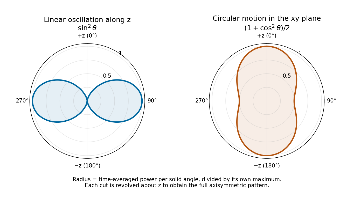
Normalized angular power for linear oscillation and nonrelativistic circular motion, with angle measured from the same z axis
. Details. 
Treat a single weakly driven Electron or an independent bound charge, so that the incident electric field is approximately uniform across its displacement. The classical calculation uses electric dipole radiation and excludes both a resonant divergence and substantial quantum recoil.
In Rayleigh scattering, a small bound system develops an induced electric dipole moment . Well below its binding resonances, the electric polarizability is approximately its static value , independent of frequency. The mean radiated power and incident light intensity areDividing gives the total scattering cross sectionThis Rayleigh scattering wavelength dependence comes from the two time derivatives of an oscillating electric dipole moment, whose radiated field is proportional to . It requires the same scatterer with approximately constant low-frequency electric polarizability; resonances and strong optical dispersion invalidate the simple fourth-power law.
Thomson scattering describes the low-recoil scattering of electromagnetic radiation by a free charge. For charge and mass , the weak incident field gives peak acceleration . The mean Larmor formula power is thereforeThere is no binding force to introduce a characteristic frequency. Dividing by the same incident light intensity gives the Thomson cross-section:For an Electron, the length inside parentheses is the classical electron radius. The cross section has units and is independent of wavelength in this classical limit. The driven velocity must remain small compared with , and must make Compton recoil kinematics negligible.
Put , where is the binding spring constant rather than an optical wavenumber. The steady complex amplitude solution of the forced Lorentz oscillator model isThe acceleration complex amplitude is . HenceThis is the scattering cross-section of a harmonically bound charge. The displacement and induced electric dipole moment are parallel to the incident linear polarization, and integrating their dipole radiation over all directions gives the total cross section above.
For , binding dominates andrecovering Rayleigh scattering with static electric polarizability . For , inertia dominates: , so its second time derivative becomes frequency independent andThis is a classical Thomson scattering regime only while . Exactly at , an undamped driven oscillator has no finite steady-state amplitude; the divergent formula must not be used. Finite damping and radiation reaction regulate the physical resonant response. Coherent contributions from many charges in an extended medium can also require a structure calculation rather than multiplying this single-charge result by a particle count.
A distinct classical Thomson scattering window requires two separated scales:To remove that window, the binding frequency must be comparable with or greater than the Compton scattering recoil scale. Thus the formal condition for bound-electron scattering without a Thomson frequency window isUsing the stipulated approximate electron mass , and givesThe dimensions are . The inequality denotes a scale comparison, not a uniquely specified spring constant or a sharp transition.
There is also a physical limitation to the question's premise. Compton scattering does not begin discontinuously at ; recoil corrections grow as photon energy approaches the rest energy. If , the assumed nonrelativistic binding model is itself no longer reliable. The calculation therefore locates where no well-separated classical Thomson scattering range exists; it cannot establish a literal direct transition of a real strongly bound system using this oscillator equation alone.
First prove the two electromagnetic field invariants from the supplied three-dimensional transformations. Then distinguish the correct covariant transversality of a vacuum plane wave from the index and equivalence issues in the original tensor statement.
Let be the boost velocity, and decompose the fields into components parallel and perpendicular to it. The parallel components are unchanged. The perpendicular components obeyAll vectors inside these expressions are perpendicular to . Thus , and similarly for . In the difference of squares, the mixed terms cancel becauseIt follows thatAdding the unchanged parallel components provesFor the mixed dot product, expand directly. The terms and vanish. The remaining cross-product identity isHenceParallel-perpendicular mixed dot products are zero in both frames, soRotations also preserve these two expressions, completing the proof for proper Lorentz transformations. The second expression is a pseudoscalar under spatial parity, but is invariant under the boosts at issue here.
These results also follow from tensor contractions. In the convention used below, and . The numerical sign of the latter depends on the chosen orientation of the dual electromagnetic field tensor, while its invariance under proper Lorentz transformations does not.
Write a nonzero vacuum plane electromagnetic wave with wavevector , where is a unit propagation direction. Its propagation Lorentz four-vector is , or, up to a scalar normalization in any one frame, . It is null because .
Choose coordinates and Minkowski metric . With the supplied three-dimensional boost formulas, a consistent convention assigns the printed array to upper-index components,The index conventions for the electromagnetic field tensor then require and when both indices are lowered. The printed lower-index label therefore cannot be kept together with its electric signs and a forward propagation vector in this convention.
This is not merely an arbitrary overall sign. For a valid forward wave with , and , multiplying the printed array, unchanged, by gives an component , rather than zero. One consistent repair is to retain the printed array as and contract with . Equivalently, lower both tensor indices before forming the contraction asked for in the question.
Using that corrected lower-index tensor givesTo establish both electric and magnetic transversality, include the dual electromagnetic field tensor. Choose and ; lowering both indices then givesThe source-free plane-wave Maxwell equations are precisely the pair of covariant conditionsTheir temporal components give and . Their spatial components give the associated amplitude and orientation relations, and .
To see the Lorentz covariance explicitly, let . It is a covector, so if in one inertial frame, its Lorentz transformation is also zero in every other inertial frame. The same is true of . Since the transformed wave still has and , their temporal components implyHere , rather than a vector renormalized to have temporal component one in every frame, is the actual Lorentz four-vector; multiplying a zero contraction by a nonzero normalization does not affect the argument.
Finally, the two scalar perpendicularity statements alone are not equivalent to one tensor contraction. They do not enforce the amplitude relation between and . Conversely alone cannot exclude a longitudinal magnetic field: adding leaves its cross product unchanged. For a genuine source-free plane electromagnetic wave, the remaining Maxwell equations supply that missing constraint, and both tensor contractions vanish. This qualification and the corrected index placement are necessary for the intended invariance argument.
Articles by others on the same topic
There are currently no matching articles.