Past exam of the physics A course of the University of Cambridge / 2022 / Paper 1

Let the infinite outer walls be at $x=0,D$, the finite steps at $x=a,b$, and the three potential energy values be $V_L,V_B,V_R$. The original drawing specifies the orderingThe energy eigenstates can be chosen real. The Dirichlet boundary conditions are $\psi (0)=\psi (D)=0$; wavefunction matching at a finite potential step requires both $\psi$ and ${\psi }^{\prime }$ to be continuous at $a,b$. In particular, neither finite step acts as an additional hard wall.

The Time-independent Schrödinger equation givesThus a wavefunction is sinusoidal in a classically allowed region, with wavenumber $k=\sqrt{2m(E-V)}/\hslash$, and a linear combination of exponential functions in a classically forbidden region, with inverse decay length $q=\sqrt{2m(V-E)}/\hslash$. Its curvature changes sign relative to $\psi$ at a step crossing $E$; its slope does not jump.

By the Sturm oscillation theorem, the three energy eigenstates have exactly zero, one, and two interior nodes, respectively. Choose their global phases so that their slopes at the left wall are positive:

For $E_0,E_1$, the right-hand piece is proportional to $\sinh [q_R(D-x)]$, rather than a pure decaying exponential: this enforces the finite-distance hard wall exactly. The barrier pieces likewise contain both exponential solutions. Their small tails are an instance of quantum tunnelling.

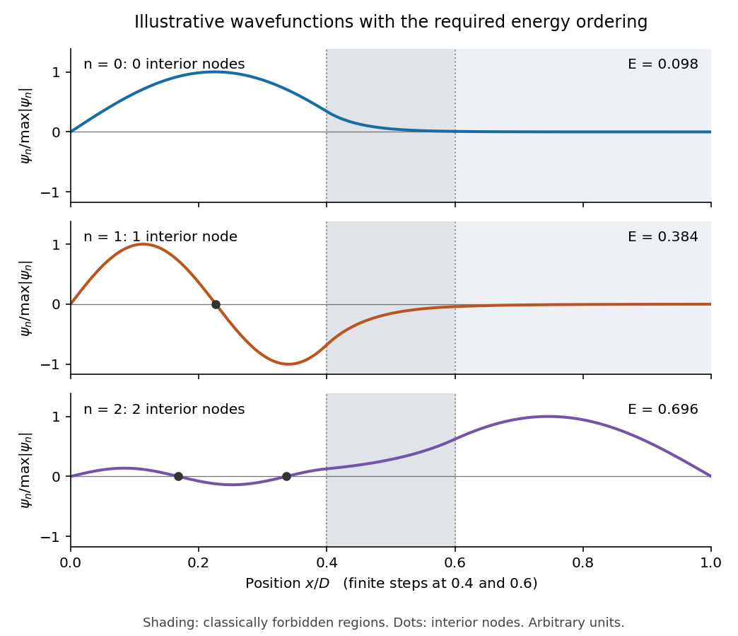
This is an original illustrative calculation, with vertical lines marking only the region boundaries. It uses $D=1$, $a=0.4$, $b=0.6$, $V_L=0$, $V_R=0.62$, $V_B=0.82$, and ${\hslash }^2/(2m{D}^2)=0.002$ in arbitrary energy units. Its lowest energy eigenvalues are approximately $0.098,0.384,0.696$, so it has exactly the required ordering. Here both nodes of the third wavefunction happen to lie towards the left; its dominant lobe is on the right. These precise positions and relative amplitudes are illustrative: the original drawing supplies no numerical lengths, barrier heights, or mass, so it does not determine a unique quantitative wavefunction. The required sketch features are the matching, curvature, hard-wall zeros, and ordered node counts.

The protons at the Large Hadron Collider are ultrarelativistic: their energy is much greater than their rest energy, about $0.938\mathrm{GeV}$. The relativistic energy-momentum relation therefore gives $pc\simeq E$. Using the de Broglie wavelength,Thus the conventional de Broglie wavelength estimate is a distance of order $10^{-19}\mathrm{m}$.

There is a conventional factor of $2\pi$ in interpreting this estimate. Spatial resolution from momentum transfer is often expressed as $\ell \sim \hslash c/Q$, where $Q$ is the transferred momentum multiplied by the speed of light. Taking $Q$ of order the beam energy givesBoth conventions describe the same characteristic scale up to $2\pi$. The beam energy alone does not give an exact experimental spatial resolution: a particular collision probes a scale set by its actual momentum transfer.

The Born rule uses the squared modulus of the wavefunction, not its real part. Write $\psi =A[\sin x+i(1-\cos x)]$. ThenWavefunction normalization requiresIntegrating the probability density over the required interval gives the dimensionless probabilityThus approximately $9.08\%$ of position measurements fall in this interval.

Let $M$ denote an incident muon and $S$ a detector signal. The selected sample is conditioned on $S$. The law of total probability givesBy Bayes' theorem, the contamination, namely the conditional probability that a selected particle is not a muon, isFor example, per $10000$ incident particles the expected selected counts are $8550$ true muons and $100$ other particles. The denominator is the $8650$ selected particles; the rejected muons are outside this sample.

For the $110\mathrm{Hz}$ fundamental alone, the Nyquist–Shannon sampling theorem places the limiting sampling rate at twice that frequency:Use a rate strictly above this boundary for a sinusoid of unknown phase: exactly two samples per cycle can, for a particular phase, all fall at zero. If higher Fourier harmonics are retained, the sampling rate must instead exceed twice the highest retained frequency, or those components must be removed to prevent aliasing.

For a straightforward discrete Fourier transform estimate, Fourier frequency resolution obeys $\Delta f\sim 1/T_{\mathrm{obs}}$. Resolving $0.07\mathrm{Hz}$ therefore suggestsAt the limiting sampling rate this is about $f_s{T}_{\mathrm{obs}}\simeq 3143$ samples. These are the usual sampling and spectral-resolution estimates. The $14.3\mathrm{s}$ value is not a universal lower bound on single-tone frequency estimation: fitting a sinusoidal model with sufficiently low noise can estimate its frequency more precisely than the spacing of discrete Fourier transform bins. The question gives no noise level or estimator, so a sharper universal minimum time cannot be deduced.

Use the canonical commutation relations $[\hat{x},{\hat{p}}_x]=[\hat{y},{\hat{p}}_y]=i\hslash$, with cross-coordinate commutators zero. For either coordinate,Thus $2\alpha \beta \hslash =1$. To obtain the required Hamiltonian, the ratio of its position operator and momentum operator coefficients must be preserved:where the positive root follows from the requested signs. ConsequentlyThe annihilation operators are dimensionless; $\alpha$ has units of inverse length and $\beta$ has units of inverse momentum. Operators belonging to different coordinates commute automatically. Writing the number operators as ${\hat{N}}_j={\hat{a}}_j^{†}{\hat{a}}_j$, substitution givesThe constant is the sum of the two zero-point energies of this two-dimensional isotropic harmonic oscillator.

For either number operator $\hat{N}={\hat{a}}^{†}\hat{a}$, positivity follows fromHence an eigenvalue $\nu$ cannot be negative. The commutatorsshow that $\hat{a}|\nu ⟩$, if nonzero, is an eigenstate with eigenvalue $\nu -1$. For a normalized eigenstate, $\Vert \hat{a}|\nu ⟩{\Vert }^2=\nu$.

If $\nu$ were not an integer, successive nonzero lowerings would eventually reach an eigenstate with $0<{\nu }^{\prime }<1$. Its next lowering would have nonzero norm but a negative eigenvalue, contradicting positivity. The ladder must therefore terminate at $\nu =0$, with $\hat{a}|0⟩=0$. Conversely, successive applications of the creation operator never vanish, becauseThe normalizable bottom state exists explicitly: solving $\hat{a}{\psi }_0=0$ gives ${\psi }_0(x)\propto \exp [-m\omega x^2/(2\hslash )]$. Thus the number operator has exactly the non-negative integer eigenvalues.

Since the two coordinate number operators commute, use the product eigenstates $|n_x,n_y⟩$. Their energy eigenvalues areAt fixed $N=n_x+n_y$, the allowed pairs are $(0,N),(1,N-1),\dots ,(N,0)$. Thus the energy level $E_N=(N+1)\hslash \omega$ has quantum degeneracy $N+1$, and the ground-state energy is $\hslash \omega$.

The number operator commutators established above imply that ${\hat{a}}_x^{†}|n⟩$ is proportional to $|n+1⟩$ and ${\hat{a}}_x|n⟩$ to $|n-1⟩$. Their norms determine the magnitudes of the proportionality constants:Choose the phase of the normalized ground eigenstate once, then define recursivelyThis removes the otherwise arbitrary relative phases of the eigenstates. The Hermitian adjoint relation then fixes the lowering coefficient with the same positive sign, givingAt $n=0$, the second expression means the zero vector, ${\hat{a}}_x|0⟩=0$; it does not introduce a physical state $|-1⟩$.

Set $\hat{B}={\hat{a}}_x^{†}{\hat{a}}_y-{\hat{a}}_y^{†}{\hat{a}}_x$. Taking the Hermitian adjoint reverses the order of products, so ${\hat{B}}^{†}=-\hat{B}$. Complex conjugation also reverses the sign of $-i$, and thereforeThus $\hat{Q}$ is a self-adjoint operator on the usual oscillator states.

Using the coefficients in part (a), products containing two position operators or two momentum operators cancel in the difference. Cross-coordinate operators commute, leavingHenceIt is the component of orbital angular momentum perpendicular to the plane, with units $\mathrm{kg}{\mathrm{m}}^2{\mathrm{s}}^{-1}$ (equivalently $\mathrm{J}\mathrm{s}$). The rotational symmetry of the two-dimensional isotropic harmonic oscillator makes this a conserved observable; directly, each term in $\hat{B}$ preserves $N_x+N_y$, so $[\hat{H},\hat{Q}]=0$.

The specified energy requires $n_x+n_y=2$, so the relevant energy eigenspace has the orthonormal basisApplying the creation and annihilation operators givesThus its matrix in this ordered basis isWriting $q=\hslash \lambda$, the characteristic polynomial gives $\lambda ({\lambda }^2-4)=0$. The possible angular momentum eigenvalues are thereforeFor completeness, normalized simultaneous energy and angular momentum eigenstates areEach value occurs once in this energy eigenspace. Equivalently, circular ladder operators of a two-dimensional oscillator give $\hat{H}=\hslash \omega ({\hat{N}}_{+}+{\hat{N}}_{-}+1)$ and ${\hat{L}}_z=\hslash ({\hat{N}}_{+}-{\hat{N}}_{-})$. With $N_{+}+N_{-}=2$, the difference can only be $2,0,-2$.

For a particle in a ring, the arc-length coordinate is $s=R\varphi$. The tangential kinetic energy isThe constraint removes radial motion; the constant potential energy along the ring can be chosen as zero. The tangential momentum operator is ${\hat{p}}_s=-i\hslash {\partial }_s$, or equivalently the angular momentum operator is ${\hat{L}}_z=-i\hslash {\partial }_{\varphi }$. ThusIts physical domain has periodic boundary conditions, $\psi (\varphi +2\pi )=\psi (\varphi )$ and ${\psi }^{\prime }(\varphi +2\pi )={\psi }^{\prime }(\varphi )$. These make the Hamiltonian self-adjoint and reflect that $\varphi$ and $\varphi +2\pi$ describe the same point. No magnetic flux or additional angle-dependent potential energy is present.

Solving the Time-independent Schrödinger equation with $\psi \propto e^{ik\varphi }$ gives $E={\hslash }^2{k}^2/(2m{R}^2)$. The periodic boundary condition requires $e^{2\pi ik}=1$, hence $k=n\in \mathbb{Z}$. With the angular integration measure $d\varphi$, wavefunction normalization givesso a convenient orthonormal eigenbasis isThe $n=0$ ground state is nondegenerate. For each $|n|>0$, $u_n$ and $u_{-n}$ span a two-dimensional energy eigenspace; real sine and cosine combinations are an equally valid basis. These opposite-circulation eigenstates have angular momentum $n\hslash$ and $-n\hslash$.

If instead the wavefunction is normalized with respect to physical arc length $ds=Rd\varphi$, its expression is $e^{in\varphi }/\sqrt{2\pi R}$. The two conventions describe the same probability, since $|u_n{|}^{2}d\varphi =|u_n/\sqrt{R}{|}^{2}ds$. The remaining parts use $d\varphi$.

Put $ϵ={\hslash }^2/(2m{R}^2)$. The two-particle product energy eigenstates areBecause the particles are distinguishable, $(n_1,n_2)$ and $(n_2,n_1)$ are distinct when $n_1\ne n_2$. Also, the signs of nonzero integers distinguish opposite angular momenta. The quantum degeneracy is therefore the number of ordered integer pairs at each sum of squares.

The first distinct energy levels are $0,ϵ,2ϵ,4ϵ,5ϵ,\dots$. This ordering matters: $4ϵ$ is the third excited level, while $5ϵ$ is the fourth excited level.

These counts concern energy eigenspaces; arbitrary quantum superpositions within each one do not create additional independent states.

Identical spin one-half particles are fermions. By fermionic exchange symmetry, the complete spatial-and-spin wavefunction must change sign when the two particle labels are exchanged. Define the normalized antisymmetric spin-one-half singlet stateand the three symmetric spin-one-half triplet statesThe Hamiltonian is independent of spin, so these spin functions carry no additional energy.

Both particles can occupy $u_0$ if their spin factor is antisymmetric. The unique ground state wavefunction isTwo equal-spin particles could not share this orbital, by the Pauli exclusion principle.

At the first excited energy, $E=ϵ={\hslash }^2/(2m{R}^2)$, one orbital is $u_0$ and the other is $u_s$ with $s=+1$ or $-1$. Define symmetric and antisymmetric normalized spatial functionsFor each $s$, all allowed wavefunctions are spanned byThere are $2(1+3)$ orthonormal states, hence first-excited-state degeneracy $g=8$. In each product, exactly one factor is antisymmetric, ensuring the required total fermionic exchange symmetry.

The original apparatus has two small masses at distance $L/2$ from the suspension axis. Neglecting the rod's moment of inertia, their total moment of inertia is $I=2m(L/2{)}^2=m{L}^2/2$, consistent with the supplied torsion pendulum period. Treat $m$ and $L$ as exact because no uncertainties are specified. Rearranging the period relation givesThe torsion constant is a restoring torque per unit angle. In dimensional calculations the radian is dimensionless.

Using first-order propagation of uncertainty, with the quoted period uncertainty interpreted as a standard uncertainty,Consequently

Rearrange the given torsion balance equilibrium relation asA useful choice, preserving equal measurement uncertainties on the vertical axis, isWith angle measured in radians, $y$ is dimensionless and $x$ has units ${\mathrm{m}}^{-2}$, so $c$ has units ${\mathrm{m}}^2$, as required. The four $x$ values, in the order of the original table, areThe corresponding $y$ values are $(0.066,0.055,0.044,0.025)$, each with standard uncertainty ${\sigma }_y=0.002$. The uncertainty of $x$ is negligible by assumption, making linear regression through the origin appropriate for the proposed model.

All four angle measurements have the same standard uncertainty, so ordinary least squares minimizesDifferentiation givesThus the unique minimum isThe overbars denote sample means over the four observations. Numerically,soThe fixed $x_i$ have negligible uncertainty. Assuming independent errors in the four $y_i$, propagation of uncertainty in quadrature givesHenceIf the period measurement is independent of the angle measurements, including its calibration uncertainty givesThis last uncertainty includes the stated random measurement errors only. Whether the model describes the data must be checked before treating it as a reliable measurement of the gravitational constant.

Assume independent normally distributed angle errors with known standard deviation ${\sigma }_y=0.002$. The relevant chi-squared test uses the sum of squared standardized residuals,For the model through the origin, the predictions and residuals, expressed in milliradians, areConsequently ${\chi }_0^2=30.0280$. There are $4-1=3$ statistical degrees of freedom. The upper-tail P-value is approximately $1.36\times 10^{-6}$; equivalently the value greatly exceeds the $5\%$ critical value $7.815$. The zero-intercept model is strongly rejected under the stated errors.

For the alternative linear regression, minimize ${\sum }_i(y_i-c^{\prime }{x}_i-d{)}^2$. Setting both partial derivatives to zero gives the normal equations, whose solution isFor these data $\bar{x}=2508.83699{\mathrm{m}}^{-2}$, $\bar{y}=0.0475$, and $S_{xx}=4.830232\times 10^6{\mathrm{m}}^{-4}$. This yieldsThe new predictions are $(66.6548,55.4171,41.4315,26.4966)\mathrm{mrad}$, with residuals $(-0.6548,-0.4171,2.5685,-1.4966)\mathrm{mrad}$. ThereforeThe affine model is compatible with the data. Allowing for its additional fitted parameter, the decrease $\Delta {\chi }^2=27.668$ has a chi-squared distribution with one statistical degree of freedom under the nested zero-intercept hypothesis, corresponding to $p\simeq 1.44\times 10^{-7}$. Thus the model with a fitted intercept provides the better description, rather than merely lowering the residual by adding a parameter.

With the measurement variance treated as known, the coefficient uncertainties areHence $d=(13.11\pm 2.49)\mathrm{mrad}$, about $5.26$ standard deviations above zero. A positive constant systematic error in the angular zero, or an additional nearly constant torque, could account for it. Its presence is evidence against the ideal zero-intercept model; four points alone do not identify the physical cause uniquely. A calibration error in $\kappa$ only rescales the inferred gravitational constant and cannot remove this residual pattern.

Using the fitted slope after allowing for this offset would give $G^{\prime }=\kappa {\hat{c}}^{\prime }/(mML)=(7.27\pm 0.51)\times 10^{-11}{\mathrm{m}}^3\mathrm{k}{\mathrm{g}}^{-1}{\mathrm{s}}^{-2}$, with the period and slope errors combined in quadrature. This is conditional on the constant-offset model.

Time dependence in quantum mechanics describes how a prepared quantum state changes and thereby changes the probabilities of later measurements. For an isolated system, the Schrödinger picture assigns this evolution to a state vector $|\psi (t)⟩$, governed by the Time-dependent Schrödinger equationThe Hamiltonian is a self-adjoint operator; it has units of energy, while $\hslash$ has units of action, so $\hat{H}/\hslash$ has units of inverse time. For a particle with potential energy $V(\mathbf{r},t)$, this becomesGiven a suitable initial wavefunction and the physical boundary conditions, this first-order equation determines its subsequent propagation. Its linearity means that the evolution of a quantum superposition is the corresponding quantum superposition of evolved states.

For a real potential energy, this equation and its complex conjugate imply the local continuity equationHere $\rho$ is the probability density and $\mathbf{j}$ the probability current. Vanishing net boundary flux preserves wavefunction normalization, as required by the Born rule.

The time-evolution operator packages the solution for every initial state:Because ${\hat{H}}^{†}=\hat{H}$, differentiation givesTherefore $U^{†}U=I$: this is unitary time evolution, preserving inner products and all state norms. It is reversible, with $U(t,t_0{)}^{-1}=U(t_0,t)=U(t,t_0{)}^{†}$, and obeys the composition law $U(t_2,t_0)=U(t_2,t_1)U(t_1,t_0)$.

For a time-independent Hamiltonian, the solution is the operator exponentialIf the Hamiltonian varies with time, the analogous simple exponential of its integral is valid when $[\hat{H}(t),\hat{H}(t^{\prime })]=0$ for all relevant times. Otherwise time ordering is essential:The meaning is explicit in the first terms of the ordered series,the later-time operator stands on the left. In the position representation, the same propagation is expressed by the quantum-mechanical propagatorIts initial value is the Dirac delta function ${\delta }^3(\mathbf{r}-{\mathbf{r}}^{\prime })$.

A time-independent Hamiltonian has energy eigenstates satisfying $\hat{H}|n⟩=E_n|n⟩$. A single such initial state evolves asIt is a stationary state: its global phase changes, but its probability density and the distributions of time-independent observables do not. Its energy is sharp. Any quantum superposition entirely within one degenerate energy eigenspace also acquires one common global phase and is stationary. Stationarity does not require zero probability current; for instance, $u_n(\varphi )=e^{in\varphi }/\sqrt{2\pi }$ on the ring has a constant density and persistent circulation when $n\ne 0$.

An arbitrary normalized state can instead contain different energy eigenvalues:A continuous spectrum requires corresponding integrals. For the discrete case, an energy measurement gives $E_n$ with fixed probability $|c_n{|}^2$ (summed over degeneracies), but relative quantum phases change with time. ConsequentlyThe interference terms can oscillate at angular frequencies $(E_m-E_n)/\hslash$. For two populated energy levels, this supplies a characteristic period $2\pi \hslash /|E_m-E_n|$ when the interference term is nonzero. Thus fixed energy populations do not imply a stationary spatial distribution.

For a normalized state and an observable $\hat{A}(t)$, its expectation value isThis is the statistical mean over repeated preparations and measurements. In an eigenbasis of energy eigenstates for a time-independent Hamiltonian and a time-independent $\hat{A}$,Only matrix elements connecting different energies can generate these oscillations. If $[\hat{A},\hat{H}]=0$, its expectation value is constant for every initial state, provided it has no explicit time dependence.

Differentiating the expectation value and substituting the Schrödinger equation for both the bra and ket proves the general Ehrenfest theorem:Equivalently,These manipulations require the state to lie in the relevant operator domains. Taking $\hat{A}=\hat{H}$ gives $d⟨H⟩/dt=⟨{\partial }_t\hat{H}⟩$, so energy is conserved under a time-independent Hamiltonian.