At coexistence, the two phases have equal chemical potential. For a single component, , with entropy and volume measured on the same molar or mass basis. Equating the phase derivatives along coexistence gives . Reversible latent heat satisfies , henceHere and are coexistence pressure and absolute temperature, is latent heat for transforming phase 1 to phase 2, and uses the same amount of material as .
For vaporization, neglect liquid molar volume compared with ideal-vapour volume . The ideal-vapour Clausius-Clapeyron approximation becomesUsing the normal boiling reference , and the supplied constant givesThis deliberately constant-latent-heat extrapolation does not reproduce the supplied triple-point pressure exactly. It predicts the liquid-vapour branch, metastable against ice below the triple-point temperature; it is not a precision sublimation-pressure prediction.
The phase diagram has solid, liquid and vapour regions meeting at the triple point. The sublimation and vaporization boundaries have positive slopes, whereas the ordinary ice–water boundary slopes negatively because ice has larger specific volume. The liquid–vapour line terminates at a critical point; the original schematic below emphasizes topology and marks the supplied triple point.
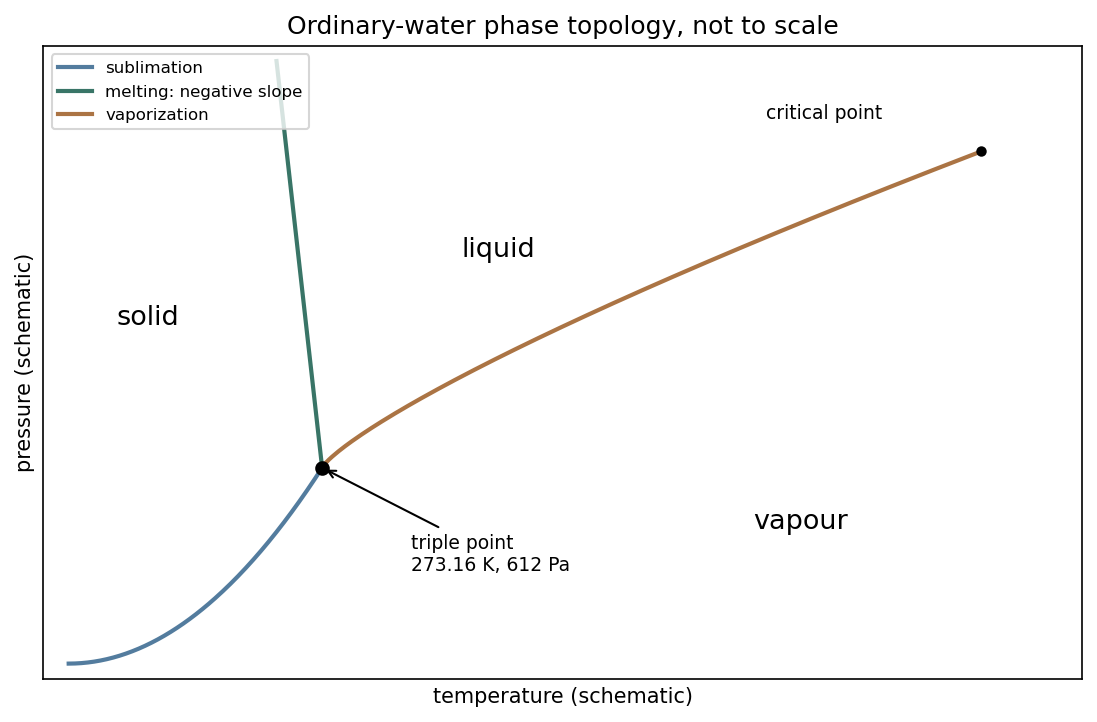
Schematic pressure–temperature phase topology of ordinary water, with negative melting slope and the supplied triple point
. Details. 
For the melting-pressure estimate, Archimedes' principle gives , soConvert the molar evaporation heat using water molar mass , rounded from the tabulated value .[ref] An enthalpy cycle through vapour then givesThis uses the question's temperature-independent evaporation heat all the way to the triple point; no replacement experimental fusion heat is inserted. The melting pressure inferred from flotation and latent heats, on holding and constant, isusing and . Linearizing the logarithm about the triple point gives instead of . Both are estimates within the stated constant-property approximation; the negative melting slope makes a positive pressure necessary to lower the melting temperature.
Capacity convention. The printed equation requires to be volumetric heat capacity, in . If “specific heat capacity” means per unit mass instead, the storage term is and both denominators in the printed equation must contain . This distinction is fixed by dimensions.
For a fixed material region , conservation of thermal energy gives the heat balance with volumetric heat generation,Use the divergence theorem, and constant coefficients. Since the region is arbitrary,The heat source is power per volume, while is thermal conductivity rather than thermal diffusivity.
For uniform electrical conductivity and imposed current, current density is and Joule heating is . A long, steady, cylindrically symmetric wire therefore satisfiesIntegration gives . Regularity at makes , and the surface condition fixes the remaining constant. Thus the Joule-heated cylindrical wire hasHere denotes the printed radial coordinate and avoids confusing it with mass density. The centre is hotter by .
For the air boundary, the internal flux at is . Equate this to . The Newton cooling of a Joule-heated wire givesMultiplication by circumference verifies that surface loss per length equals , the electrical power per length. The full air-cooled profile uses this surface temperature plus the same parabolic interior excess, assuming constant material properties and negligible end losses.
A heat engine's thermal efficiency is net work out divided by heat absorbed,where both heat quantities are positive magnitudes. The last equality follows from the first law over a complete cycle.
Use moles of an ideal gas with constant molar and . For the Otto cycle, reversible adiabats give and . Isochoric heat input and rejection are and . ThereforeThe denominator's temperature difference is times the numerator's difference.
For the ideal Atkinson cycle, heating at fixed volume gives . The longer expansion ends when . Combining the adiabatic pressure–temperature relation with yieldsAlso for . The PDF asks explicitly for ; the transcription additionally names , which is supplied above too.
Heat input remains , while the isobaric return rejects . Hence the Atkinson efficiency advantage from extended expansion is quantified byCompare cycles with the same initial state, compression ratio and heat input. The extra expansion and constant-pressure return enclose positive extra work,It uses heat that the Otto cycle would reject, while is unchanged. Equivalently, concavity gives , so for under this matched comparison. This is an ideal-cycle result; the question's named real-engine application is not needed to establish it.
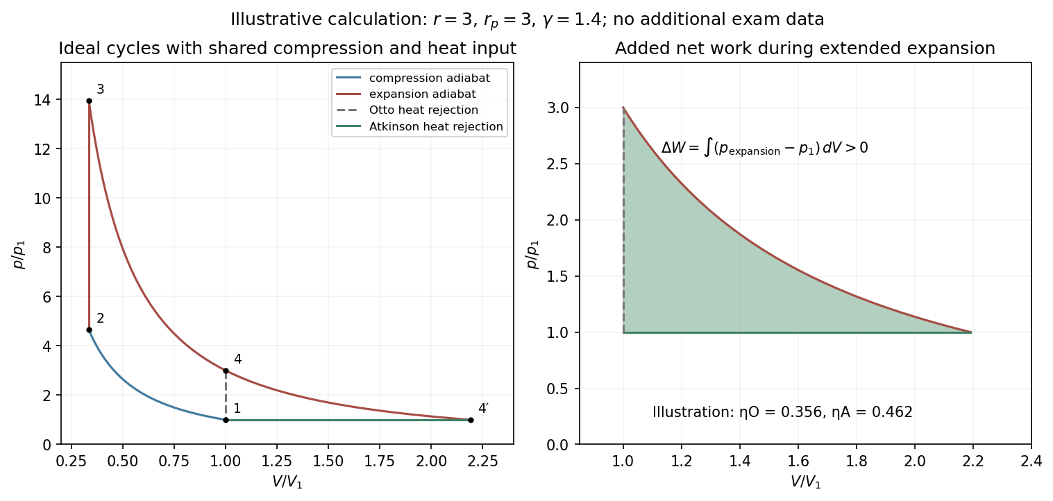
Original ideal-gas cycle calculation showing the extra expansion work and the matched Otto–Atkinson efficiency comparison
. Details. 
For a simple compressible one-component equilibrium system, the fundamental thermodynamic relation isThe internal energy has natural variables : its derivatives give , and chemical potential . The natural variables of a thermodynamic potential identify the independent arguments whose conjugates appear directly in a potential's differential. A Legendre transform exchanges a variable for its conjugate, giving potentials suited to different controlled conditions:
| potential | definition | natural variables | differential |
|---|---|---|---|
| internal energy | |||
| enthalpy | |||
| Helmholtz free energy | |||
| Gibbs free energy |
For fixed composition and the appropriate closed-system constraints, equilibrium minimizes at fixed , at fixed , at fixed , or at fixed , with other allowable internal variations understood. Enthalpy is useful for constant-pressure heat exchange with only pressure–volume work. Helmholtz free energy is suited to fixed-temperature, fixed-volume systems, and Gibbs free energy to fixed-temperature, fixed-pressure phase or chemical equilibrium. Coexisting phases of one substance have equal chemical potentials.
Where a potential is twice continuously differentiable, equality of mixed derivatives gives Maxwell relations. At fixed , the four usual forms areThe fixed subscripts and signs follow from the chosen natural variables. Derivatives through a nonsmooth phase boundary require separate phase descriptions rather than automatic use of the smooth single-phase formulas.
As an application, the Helmholtz relation turns pressure data into an isothermal entropy change. For an ideal gas, , givingCombining the same relation with yields , which vanishes for an ideal gas and reveals attractive-energy effects for a van der Waals gas. Thermodynamic potentials organize equilibrium constraints, while Maxwell relations convert difficult entropy derivatives into measurable response derivatives.
Articles by others on the same topic
There are currently no matching articles.