Original paper: Public original, physical PDF pages 128–135.
Use absolute thermodynamic temperatures and assume a constant-parameter Arrhenius equation, with composition held fixed so that reaction rate is proportional to the rate constant. Write , where . two-temperature Arrhenius extrapolation eliminates the unknown Arrhenius prefactor and givesConsequentlyA tenfold increase for one interval does not imply another tenfold increase for the next interval: the Arrhenius plot is linear in inverse temperature. Two measured rates alone do not specify a unique extrapolation without a rate law for its temperature dependence; the result above states that modelling assumption explicitly.
Choose the plate polarity so that the gap electric field points along when . Away from the plate edges, the quasistatic electromagnetic approximation gives . A circular Ampere-Maxwell law contour of radius then givesIt is displacement current, rather than a conduction current across the air, that supplies the enclosed current term. The direction follows the right-hand rule for increasing positive electric flux; it reverses every half cycle. In the ideal extension that sets the gap electric field to zero outside the plate footprint, for . That extension is an edge approximation, not an exact exterior solution for finite plates. Neglect fringing field of a capacitor and retardation, requiring and .
For a hollow, air-filled rectangular electromagnetic waveguide with conducting walls, transverse confinement givesA transverse electric mode of a rectangular waveguide permits one zero index, but not two; a transverse magnetic mode of a rectangular waveguide requires both indices positive. Take and . The dominant mode is , withThe waveguide cutoff frequency is the limiting value: positive axial group velocity and propagating power require . There is no transverse electromagnetic mode in this single hollow conducting pipe; otherwise a zero cutoff would incorrectly follow.
The Stefan–Boltzmann law gives solar luminosity . At orbital distance , the incident irradiance is . A spherical absorber intercepts a disc of area but radiates over . Thus the uniform-temperature radiative equilibrium estimate isThe planetary radius cancels. This is a black-body radiation estimate with zero reflected fraction and complete redistribution of absorbed heat. More generally the balance fixes , rather than the arithmetic mean of a nonuniform surface temperature. It excludes atmospheric heating and thermal lag; no measured surface temperature is inferred.
For the inertia tensor of a uniform cube, reflection symmetry makes every off-diagonal element of the central inertia tensor vanish. Permutation of the three axes makes its diagonal elements equal. Since and the mean of each squared coordinate in the cube is ,Every central axis is therefore a principal axis, including the body diagonal. The angular momentum is parallel to the angular velocity, and its magnitude is
In a charge-free region of homogeneous permittivity, Gauss's law and give Laplace's equation, . Prescribed surface electric potentials specify a Dirichlet problem. Its Uniqueness of the Dirichlet problem permits replacing conductors by fictitious charges outside the physical solution region: a harmonic candidate with the same boundary conditions is the physical solution. For an exterior problem its behaviour at infinity must also be prescribed. For a proof, subtract two candidate potentials to obtain with zero boundary values. Green's first identity gives , so is constant and its boundary value fixes it to zero. Conditions on a normal electric field instead determine a potential only up to an additive constant when the usual compatibility condition holds.
A cylindrical Gaussian surface around an infinite line charge gives . The electric potential difference is thereforeAn isolated infinite line charge has no finite potential zero at infinity. For the opposite pair, however, the logarithmic growth terms cancel and one can choose there. Define and . superposition givesOn ,Thus the circle, and its cylindrical extension, is an equipotential. This is an Apollonius circle: a constant ratio of distances gives a circle rather than a constant distance from either charge.
For the cylinder above the plane, call its centre height and set . The cylinder-plane image charges are at height and at height . Their distances are equal on the grounded plane, while their distance ratio is on the circular surface. The positive fictitious line lies inside the metal, so the exterior is charge-free and Uniqueness of the Dirichlet problem applies. A Gaussian surface enclosing the physical cylinder confirms that its charge per unit length is indeed . Its voltage isThe physical field energy per unit length at fixed cylinder charge is . Differentiate with respect to height, keeping and fixed:The electrostatic attraction per unit length of a cylinder above a plane is downward for either sign of charge. Placing the fictitious line at the cylinder centre would give the wrong answer at this separation. The long-cylinder approximation neglects the ends.
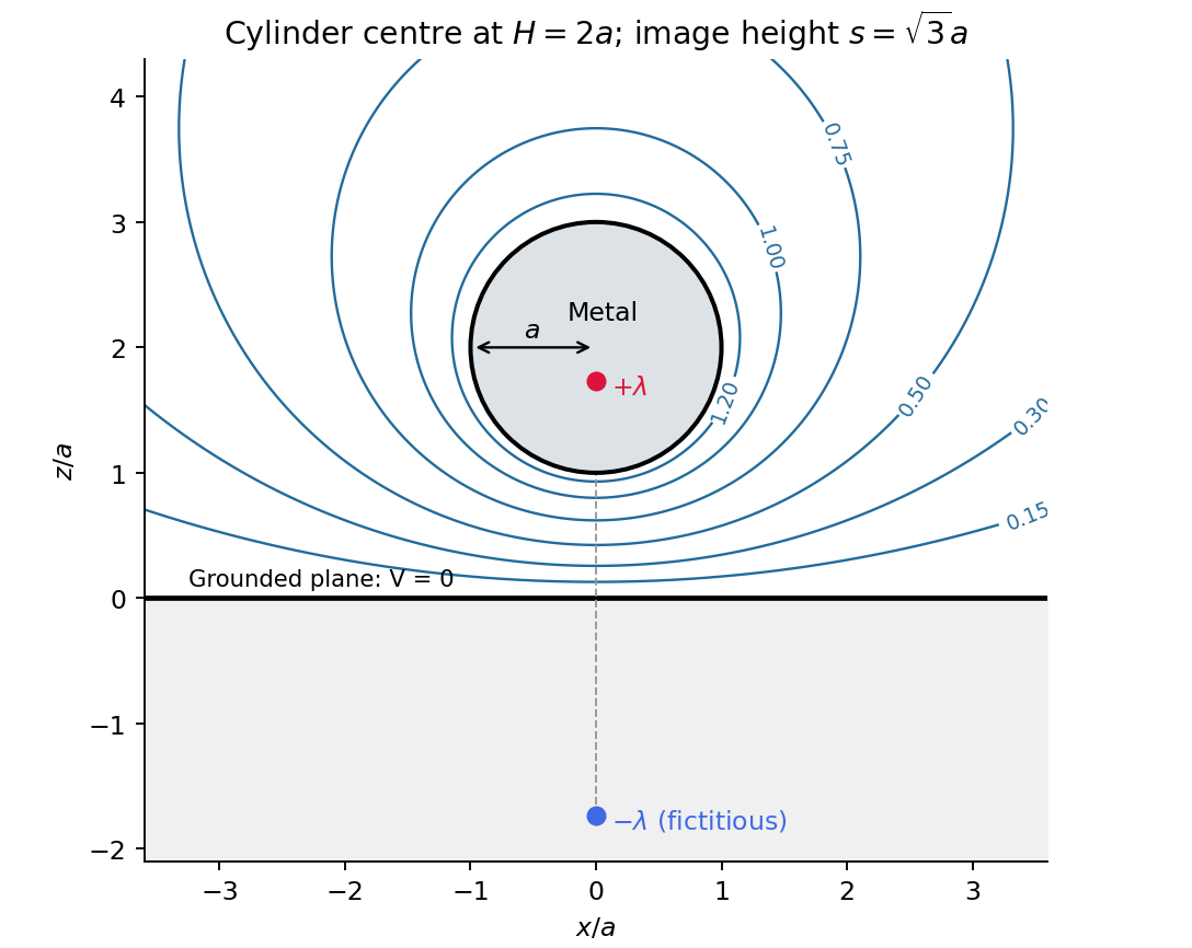
Original cylinder-plane image charges construction and exterior equipotentials
. Details. For fixed, magnetically linear geometry, self-inductance relates a coil's own magnetic flux linkage to its electric current, . mutual inductance relates the linkage in one coil to the current in the other, . These coefficients enter the induced electromotive forces through ; reversing a chosen winding orientation reverses the sign assigned to .
In the ideal confined-field toroid, a circular magnetostatic Ampère law contour encloses , soWrite for the height of the square cross-section. The inductance of a rectangular-section toroid follows by integrating the magnetic flux density over that cross-section; it cannot be replaced by its value at an arbitrary mean radius:Consequently, for winding normals chosen consistently,The equality means complete shared magnetic flux linkage; with leakage one instead has .
For the crack, use the radial-path approximation for a cracked toroid, with an air length on each path and core length . Continuity of the normal magnetic flux density at a crack face gives . HenceIntegrating the radial paths yieldsHere and : about a 53% reduction. The small ratio does not justify expanding in , which is about ten. The crack's low magnetic permeability gives appreciable magnetic reluctance. This is an estimate within a confined-flux model; actual redistribution near the slit is outside its accuracy. Narrow-gap circuit models assume small gap width relative to transverse dimensions and approximately directed flux.[ref]
Magnetic Circuits. §9.7, Example 9.7.1 and the paragraph after it: air-gap circuit approximation and need for a more general field solution
For the intact ring, ideal poloidal winding currents and the no-leakage boundary condition admit with zero radial and vertical components. It is curl-free inside the current-free core, divergence-free for uniform magnetic permeability, tangent to the core boundary, and has the required circulation; uniqueness of the Neumann problem removes an additional homogeneous scalar-potential field. This explains zero non-azimuthal components in the stipulated intact-ring idealization. A literal slit breaks that rotational symmetry, so zero transverse components everywhere is not exact for the cracked ring: magnetic fringing and flux redistribution occur. In fact, extending the approximate unchanged around a current-free core would give . Thus that radial-path calculation and a claim of exact purely azimuthal field in the cracked geometry cannot both be exact. The numerical answer above retains the intended circuit approximation while making its limitation explicit.
For a steady thin-wire electric current, the Biot-Savart law iswhere the source element follows positive current. For a circular loop, source points are and the observer is . Their cross product with has axial component ; transverse components integrate to zero. Thus the on-axis magnetic field of a circular current loop, multiplied by the number of coincident turns, isTake positive current counterclockwise as seen from . magnetic field lines pass upward through the loop and return around its exterior, closing rather than terminating. They fan outward above its centre and converge below it. The original numerical Biot-Savart law integration below illustrates these directions; the wire singularities are masked.
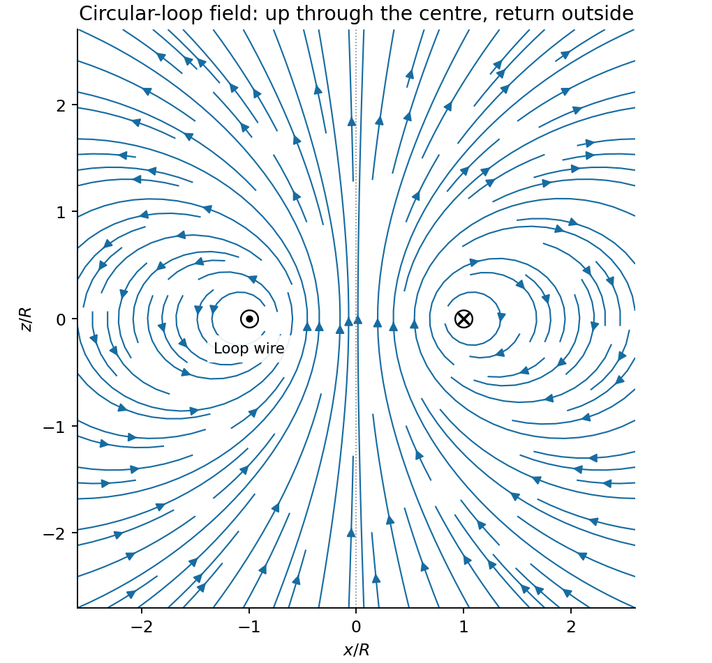
Original circular-loop magnetic field lines in a meridional cross-section
. Details. The axisymmetric magnetic field near a regular axis follows from Gauss's law for magnetism. In cylindrical coordinates, regularity gives , while symmetry gives . Integrate from the axis:A formal term is excluded by regularity. For the axial field decreases upward, so the radial component is outward, consistent with the sketch.
On the small receiving coil, . The Lorentz force has axial component . Contributions from the axial field cancel radially around the loop. ThereforeWith both currents giving magnetic dipole moments along and , this is attraction. Reversing one current reverses the force. The small coil has , so the result is exactly the leading magnetic dipole force . Equivalently . The approximation requires and negligible variation over the receiving coil; corrections begin at relative order .
Use peak-amplitude phasors with time factor and . Faraday's law of induction and the Ampere-Maxwell law giveIn the good-conductor limit , take the root with positive attenuation into the slab:The real physical field is . A thick slab excludes a returning wave from its rear face. The skin depth is the electric-field amplitude decay length; the intensity decay length is .
Faraday's law of induction fixes . The surface impedance of a good conductor and the complete transmitted magnetic field are consequentlyThe sign of the imaginary part belongs to the stated time convention. Average the Poynting vector using complex conjugation and the factor one half appropriate to peak phasors:As an independent energy check, , the mean Joule heating per unit volume.
Ohm's law gives and . Hence the averaged Lorentz force per unit volume isIntegrating through the illuminated half-space gives the positive inward radiation pressureFinally let be the vacuum wave impedance. Tangential-field boundary conditions at normal incidence give the electric-amplitude reflection coefficient . Since ,Here by surface energy balance. Combining the leading formulas gives , the nearly perfect-reflector limit. The displayed reflection expansion also assumes a good conductor relative to the incident vacuum wave, .
A normal mode is a motion in which all displacement coordinates oscillate at one angular frequency with fixed amplitude ratios. For small conservative oscillations, the symmetric stiffness and mass matrices give the generalized eigenvalue problem for small oscillations, . For positive mass and a stable equilibrium, its mass-orthogonal eigenvectors span the motion. A superposition of these modes, with phases and amplitudes fixed by initial displacements and velocities, gives the general solution; different modes need not share a phase.
Use upward end displacements. The spring compressions are and , while the beam's centre rises by . The potential energy isStatic force balance gives , cancelling the linear terms and leavingFor a uniform beam, its central moment of inertia in the vertical plane is . To first order in the tilt, . Its translational and rotational kinetic energies areThus and . The normal modes of a rigid beam on two end springs have eigenvectorsThe first translates without tilt; the second rocks about a stationary centre. Ordinary frequencies are and .
Assume the system had settled before the end load leaves, and put that load at end 1. Its extra static spring load is at that end and zero at the other. Therefore , , and both initial velocities vanish because no impulse is imparted. Decomposing into the two normal modes givesOnly the symmetric mode contributes to the centre position:The datum is the unloaded beam's equilibrium height; no absolute height is supplied. The rocking mode is present even though it cancels out of this coordinate. These results use small tilt, , ideal light vertical springs and negligible damping.
For an attractive inverse-square force, write with , and take nonzero conserved angular momentum . The conic section orbit hasThe physically allowed cases are ellipse for , parabola for , and hyperbola for . The minimum allowed energy gives the circular special case . Here is measured relative to infinity. Zero angular momentum instead gives radial collision or escape trajectories, interpreted as degenerate limits rather than regular closed ellipses.
For a repulsive inverse-square force, . The effective potential is positive and decreases from infinity to zero, so a trajectory reaching a finite radius has . For nonzero angular momentum, it is the accessible branch of a hyperbola, with . There are no bound ellipses or finite-distance zero-energy parabolas. At zero angular momentum, the motion is straight inward followed by straight outward after reflection at a radial turning point.
For the scattering calculation, take the heavy target as fixed and define . The incoming kinetic energy and angular momentum are and . In the original sketch, the horizontal dashed incoming asymptote has perpendicular distance from the nucleus, while is the radius from the nucleus to the point where .
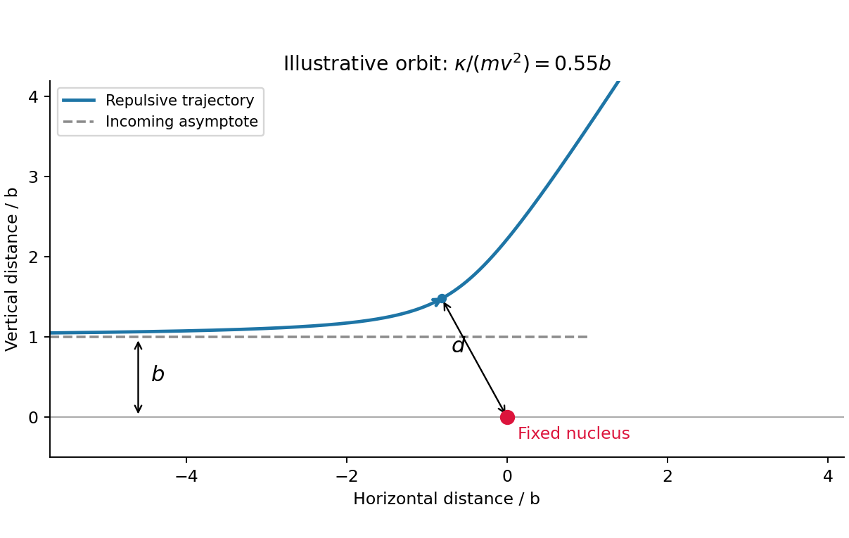
At closest approach, the velocity is tangential and . conservation of energy givesChoose the positive root and put :Head-on incidence gives , and repulsion always gives . With an attractive Coulomb force, change the sign of the potential term:For , the attractive and repulsive inverse-square closest approaches obey . For attraction causes a collision with the point centre, so is a singular endpoint, not a regular scattering turning point. Finite nuclear size is excluded by the stated point-force model.
For the repulsive inverse-cube central force , the torque vanishes, , and angular momentum is still conserved. Its potential energy is , since . ThusThe new coefficient is denoted because its units are , unlike the units of the inverse-square coefficient. Conserving angular momentum depends on centrality, not on a particular radial power law.
Measure from the upward vertical, let point from the support along the symmetry axis, and use the support as the reference point for all moments of inertia. Choose and . These form an instantaneous principal-axis frame; its transverse axes need not spin with marks painted on the body. The three infinitesimal Euler angles rotations add as vectors:Resolving the vertical direction givesA convention matters here: in genuinely material-fixed transverse axes, the first two components are rotated by the spin angle . For one conventional choice they are and . Since , that rotation changes neither kinetic energy nor the axial and vertical conserved momenta. The simplified displayed components use the instantaneous transverse frame just defined.[ref]
The Motion of Rigid Bodies. §3.5.2, angular-velocity decomposition and body-frame components; §3.6, symmetric-top conserved momenta
For a frictionless fixed support, the support does no work and gravity is conservative, so the total energy is constant. The heavy symmetric top Lagrangian isThe two cyclic coordinates giveEquivalently, gravitational torque has no component along the vertical or symmetry axis. Eliminate and the axial spin from :This is the heavy symmetric top reduction at fixed . A constant inclination must satisfy the reduced equation of motion , not merely have zero instantaneous velocity. Differentiation at fixed conserved momenta gives, for and ,Therefore uniform precession of a heavy symmetric top requiresFor a prescribed upward inclination , real precession rates exist only if the quadratic discriminant is nonnegative:For positive spin the absolute-value sign can be dropped. The two roots are the slow and fast branches and coalesce at the threshold. The familiar upright-limit critical magnitude is ; strict inequality gives gyroscopic stabilization of an inverted symmetric top. This limiting stability condition should not be confused with a positive minimum over every possible inclination. As approaches from below, the fixed-inclination threshold approaches zero. At the horizontal angle for ; below the horizontal the quadratic admits real solutions even at . The stated minimum therefore needs the inclination convention made explicit.
Use the Euler-Bernoulli beam equation for a uniform slender elastic beam, small deflection and small slope, neglecting axial tension, shear deformation, rotational inertia of a cross-section and damping. Let be Young's modulus, the second moment of area about the neutral axis, and the mass per unit length. If density instead denotes mass per volume, replace this by . The bending stiffness is ; the small-slope curvature is . The bending and kinetic energies areTwice integrating the variation of by parts gives the restoring load per unit length. Newton's second law therefore givesAt a pivot, displacement is fixed but slope is free; zero end bending moment gives . This also follows from the natural boundary term in the variation.
With separation of variables, givesChoose the time normalization . Initial rest removes the sine time term, so . The spatial characteristic roots are , givingThe two conditions at give and , hence . At , addition and subtraction of give and . Nontrivial positive-frequency modes therefore have and . Thus the simply supported beam normal modes areThe zero-frequency cubic solution also vanishes under these four endpoint conditions, so is not an additional mode.
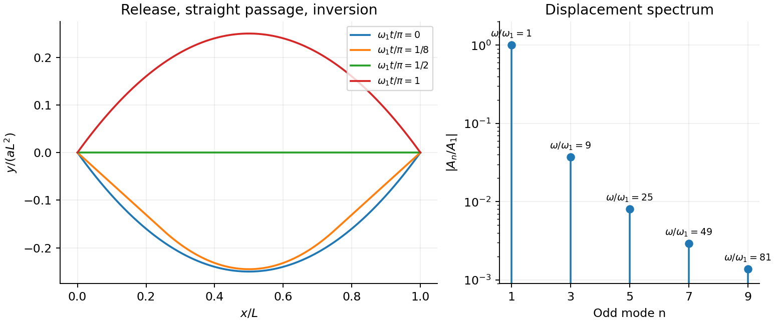
For the specified release, small slope requires . Expand the initial deflection in the Fourier sine series. Its coefficients areWriting , the resulting motion isOnly odd normal modes occur because the initial profile is symmetric about the midpoint, and their amplitudes decrease as . The frequencies grow as , so the motion is dispersive and is not a single shape multiplied by one cosine. Nevertheless the ideal undamped solution is exactly periodic with period . At all odd-mode cosines vanish, so the bar is instantaneously straight; at it has the opposite initial deflection. The first mode dominates displacement, with third-mode amplitude only of the first.
There is initial curvature incompatibility at a moment-free beam end: the prescribed parabola has , whereas a moment-free pivot requires zero curvature at an endpoint. Therefore the data do not define a classical solution with curvature continuous through the two end-time corners. They do define a finite-energy weak solution after release of the forces or end moments that prepared the initial shape. The sine expansion represents that solution: its displacement reproduces the initial parabola, each mode satisfies the released endpoint conditions, and gives finite bending energy. One must not differentiate the initial series twice at its endpoints and assign the interior parabola's curvature there. This qualification leaves the modal displacement prediction intact.


An alternate public copy is Physical pages 300–305 of the alternate source PDF.
For the one-mole convention, is the excluded molar volume: finite molecular size reduces the volume available for translational motion from to . It is an effective excluded volume, not simply the sum of the bare molecular volumes. corrects for attractive intermolecular forces, which reduce the pressure exerted on the wall. The attraction per molecule scales with number density, and the number of affected molecules also scales with density, producing the density-squared correction. The Van der Waals equation consequently raises the measured pressure to the corresponding repulsive-gas value before multiplying by the available volume. Both corrections vanish relative to the ideal-gas terms at sufficiently low density.
For inner radius and outer conductor's inner radius , Gauss's law gives . Integrating across the dielectric gives voltage . Thus the capacitance per unit length isThe stated outer radius is interpreted as the radius of the dielectric-facing surface. Magnetic permeability affects inductance, but does not enter this electrostatic capacitance.
Kepler's third law for negligible planet mass gives . Therefore . The furthest point is apoapsis, soThe supplied orbital period and eccentricity are sufficient; no present-day ephemeris is needed.
Neglect ends and take the exterior as vacuum. With polar angle measured from the applied field, regularity inside and the far-field condition allowContinuity of potential gives ; continuity of normal electric displacement, with no free surface charge, gives . Hence the transverse electrostatic field inside a dielectric cylinder is uniform, parallel to the applied field, with magnitudeThis cylindrical result differs from the spherical depolarization factor. It returns for and tends to zero for large positive .
Let be circumferential tension. A small arc subtending has inward resultant and mass . Its centripetal acceleration gives . Circumferential stress is and the strain is . Thus the centrifugal strain of a thin elastic hoop isUse the unstrained radius and cross-section at this order. The approximation requires , a slender hoop and linear elastic response; the area cancels.
A transmission line stores electric and magnetic energy along its length, so voltage and current depend on both position and time. A distributed circuit uses inductance and capacitance per length, together with resistance and leakage conductance . Applying voltage and charge balance to a short segment gives the telegrapher's equations,For a lossless line, both variables obey wave equations with speed and characteristic impedance . Forward and backward waves obey and . Matching a termination gives the voltage reflection coefficientA matched load absorbs without reflection; an open circuit has , and a short has . Reflections can produce standing waves. A coaxial line confines the fields between conductors and, for a uniform dielectric TEM wave, has . Finite loss attenuates waves; frequency-dependent losses or material properties can also distort pulses. A long line is a wave-carrying distributed system, so it cannot generally be replaced by one lumped capacitor.
Polarization density is electric dipole moment per unit volume. Displacing positive and negative bound charges leaves the bulk nearly neutral locally but can produce uncompensated charge where polarization varies or terminates. For a dielectric occupying a volume with outward unit normal ,The divergence theorem makes their total sum zero for a body described entirely by bound dipoles. Uniform polarization gives no interior volume charge but generally gives opposite surface charges on different faces.
In a linear isotropic dielectric, and . Gauss's law becomes , separating free from bound charge. Across a static interface, tangential electric field is continuous, while the normal displacement jumps by the free surface charge. Polarization charges alter the internal field, as in the dielectric cylinder calculation. Molecular distortion and orientation contribute differently, and response can depend on temperature and frequency. Bound charge is a redistribution of material charge, not an additional free-charge reservoir.
Paramagnetism has positive susceptibility: permanent spin or orbital moments tend to align with a field against thermal disorder. Independent localized moments in the classical weak-field regime give , the Curie law. Conduction-electron Pauli paramagnetism has a different origin and need not follow that temperature law.
Diamagnetism is the induced magnetic response opposing the applied field, giving negative susceptibility. Changes in orbital motion underlie this response; it exists even without permanent moments. It is often relatively weak and only weakly temperature dependent, although particular quantum systems have stronger or more complicated behaviour.
Ferromagnetism arises from interactions favouring parallel magnetic order. Below the Curie temperature a domain can have spontaneous magnetization even at zero applied field. A sample can nevertheless have nearly zero net moment if differently oriented domains cancel. Domain rearrangement and rotation produce a nonlinear magnetization curve, saturation, remanence and coercivity; hysteresis dissipates energy in a field cycle. Above the ordering temperature the spontaneous order disappears, and a Curie-Weiss susceptibility is a useful mean-field approximation. The signs of weak-field susceptibility distinguish para- and diamagnetism; spontaneous order and domain dynamics distinguish ferromagnetism from independent-moment alignment.
Use a cold, unmagnetized, collisionless electron plasma with immobile ions. For an oscillating field proportional to , the electron displacement follows . Hence andThe induced polarization opposes the field because electron inertia changes the phase of its displacement. Maxwell's equations give transverse electromagnetic dispersionThus transverse waves propagate above the plasma frequency, while below it the wavenumber is imaginary and a semi-infinite lossless plasma reflects an incident wave with an evanescent interior field. In the cold electrostatic model, a longitudinal density oscillation instead has frequency .
Collisions at rate give for this time convention, introducing absorption. A background magnetic field makes the response anisotropic, and thermal motion supplies additional dispersion and static screening. The divergent zero-frequency cold collisionless formula should not be mistaken for a complete description of static Debye screening. The simple dielectric function is a dynamical electron-inertia response under stated assumptions.
In microscopic SI form, Maxwell's equations couple charge density and current density to electric and magnetic fields:Gauss's electric law expresses electric flux from charge and reduces to the inverse-square Coulomb field for a point charge. Gauss's magnetic law gives zero net magnetic flux through every closed surface; magnetic field lines do not begin or end on magnetic monopoles in this theory.
Faraday's induction law says changing magnetic flux produces a circulating electric field. For a fixed loop, its circulation is minus the rate of change of enclosed magnetic flux, explaining the sign of induction and Lenz's law. For example, changing a primary coil's electric current changes the flux through a stationary secondary coil and induces a voltage. A moving wire also has the magnetic part of the Lorentz force on its charges; the fixed-loop field equation and the full motional-emf calculation must be distinguished.
The Ampère-Maxwell law relates magnetic circulation to conduction current and displacement current. The latter is essential around a charging capacitor: a surface cutting the lead and another passing through the gap must predict the same circulation. Taking the divergence givesusing Gauss's electric law. Charge conservation therefore fixes the consistency of the time-dependent equations. In matter, the equivalent macroscopic equations use and , free sources and constitutive relations. The Lorentz force density describes exchange of momentum with charges.
In source-free vacuum, take the curl of Faraday's law and use . Both fields satisfyFor a plane wave, , and . The fields are transverse, mutually perpendicular and in phase. Their energy density and energy flux areThis is Poynting's theorem: field energy is transported and can do work on matter. Electromagnetic radiation is a propagating, energy-carrying solution of the coupled electric and magnetic field equations.
Let a frame's origin have inertial acceleration and its axes rotate with angular velocity . For position and velocity measured in that frame, Newton's law becomesThe extra terms are translational, Coriolis, Euler and centrifugal inertial forces. Centrifugal force points away from the rotation axis; Coriolis force deflects moving bodies sideways and does no instantaneous work on their relative motion, since it is perpendicular to . The Euler term appears when the rotation rate or axis changes.
For constant , centrifugal force has potential . It can be combined with a conservative real potential to find rotating-frame equilibria. The Coriolis term remains velocity dependent. These forces arise from describing acceleration in a noninertial frame; they are not additional interactions between bodies. They are essential for trajectories on rotating apparatus and for large-scale terrestrial motions. Frame-dependent terms must be included consistently with the chosen coordinates.
A small displacement in a homogeneous isotropic elastic solid obeys linear elasticity. With Lamé constants and mass density , momentum balance givesA longitudinal plane wave has displacement parallel to its propagation direction and changes local volume. A transverse wave has perpendicular displacement and produces shear. Substitution givesAn ideal fluid has no static shear modulus and cannot support this bulk transverse elastic wave. A thin rod with free lateral surfaces instead supports an extensional long-wavelength mode with speed ; its transverse contraction changes the effective stiffness, so it should not be identified with the unbounded-solid longitudinal mode.
Stress and displacement boundary conditions produce reflection, transmission, mode conversion and guided waves. Viscoelasticity and scattering can attenuate waves; finite geometry can make guided modes dispersive even when the bulk elastic constants are frequency independent. Wave speed depends on both material stiffness and the allowed deformation.
Choose body-fixed principal axes through a fixed point or the centre of mass, with principal moments . Angular momentum has components . The inertial derivative is the body derivative plus , so Euler's equations readThey avoid differentiating the rotating inertia tensor in laboratory coordinates. Torques must refer to the chosen point, and the displayed fixed moments require a rigid body.
For zero torque, laboratory angular momentum is constant, while its components can change in the body frame. Both and rotational kinetic energy are conserved. The intersections of their constant-value surfaces constrain the motion. For distinct , steady rotation about either extreme principal axis is stable against small perturbations, whereas rotation about the intermediate axis is unstable. For example perturbing rotation about axis 2 giveswhose coefficient is positive. A symmetric body has additional simplifications and can precess. Conservation of laboratory angular momentum does not imply constant body-frame angular velocity.
For conservative forces and ideal constraints that do no work, mechanical energy is constant. Work-energy balance remains useful with nonconservative forces: their power gives . In one dimension,locates accessible regions and turning points, and reduces the trajectory to a quadrature . A local minimum of potential is a stable equilibrium; a local maximum is unstable. Near a nondegenerate minimum, gives .
For a central force, conserved angular momentum reduces radial motion to an effective potential . Its extrema determine circular orbits and their radial stability. In several coordinates, small oscillations follow from the kinetic-energy mass matrix and potential Hessian through .
Energy is also central to the Lagrangian and the Euler-Lagrange equations. A time-independent natural mechanical system has conserved energy; cyclic coordinates yield additional momenta. Energy alone does not normally determine every coordinate of a multi-degree-of-freedom motion. Its value is to expose allowed motion, stability and reductions before solving the full differential equations.
A velocity field assigns a velocity to each point. Following a fluid parcel rather than holding position fixed gives the material or convective derivativeThe convective term can accelerate fluid even in a steady flow, for example as a stream narrows. Conservation of mass is ; constant-density incompressible flow has .
For an incompressible Newtonian fluid of constant density and viscosity, with conservative body-force potential per mass , momentum balance isNeglect viscosity and assume steady flow. Dotting with an element along a streamline, or using , givesThis is Bernoulli's equation: pressure work, kinetic energy and gravitational potential energy interconvert. In a connected irrotational region under the same assumptions, is the same for all streamlines. In a rotational flow it can vary between them. Viscous dissipation, pumps or unsteady motion require the corresponding modified balance; the steady inviscid expression cannot be applied indiscriminately.
Vorticity measures local fluid rotation. For constant-density incompressible flow it evolves byshowing vortex stretching and viscous diffusion. A potential flow has locally, so irrotational incompressible motion satisfies . Boundary conditions then determine flows around simple shapes. A multiply connected region can have circulation even when its local vorticity vanishes; ideal potential flow also misses no-slip boundary layers and viscous drag.
For a Newtonian fluid, shear stress is proportional to strain rate. No-slip at solid walls produces velocity gradients and dissipation. Fully developed laminar pipe flow, for example, hasThe Reynolds number compares inertial and viscous terms. Small values favour creeping-flow approximations; large values can permit thin boundary layers and turbulence, without guaranteeing turbulence in every geometry. The appropriate flow model follows from conservation laws, constitutive properties, boundaries and scale comparisons.
At coexistence, the two phases have equal chemical potential. For a single component, , with entropy and volume measured on the same molar or mass basis. Equating the phase derivatives along coexistence gives . Reversible latent heat satisfies , henceHere and are coexistence pressure and absolute temperature, is latent heat for transforming phase 1 to phase 2, and uses the same amount of material as .
For vaporization, neglect liquid molar volume compared with ideal-vapour volume . The ideal-vapour Clausius-Clapeyron approximation becomesUsing the normal boiling reference , and the supplied constant givesThis deliberately constant-latent-heat extrapolation does not reproduce the supplied triple-point pressure exactly. It predicts the liquid-vapour branch, metastable against ice below the triple-point temperature; it is not a precision sublimation-pressure prediction.
The phase diagram has solid, liquid and vapour regions meeting at the triple point. The sublimation and vaporization boundaries have positive slopes, whereas the ordinary ice–water boundary slopes negatively because ice has larger specific volume. The liquid–vapour line terminates at a critical point; the original schematic below emphasizes topology and marks the supplied triple point.
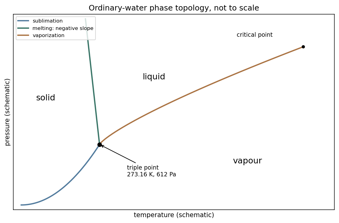
Schematic pressure–temperature phase topology of ordinary water, with negative melting slope and the supplied triple point
. Details. 
For the melting-pressure estimate, Archimedes' principle gives , soConvert the molar evaporation heat using water molar mass , rounded from the tabulated value .[ref] An enthalpy cycle through vapour then givesThis uses the question's temperature-independent evaporation heat all the way to the triple point; no replacement experimental fusion heat is inserted. The melting pressure inferred from flotation and latent heats, on holding and constant, isusing and . Linearizing the logarithm about the triple point gives instead of . Both are estimates within the stated constant-property approximation; the negative melting slope makes a positive pressure necessary to lower the melting temperature.
Capacity convention. The printed equation requires to be volumetric heat capacity, in . If “specific heat capacity” means per unit mass instead, the storage term is and both denominators in the printed equation must contain . This distinction is fixed by dimensions.
For a fixed material region , conservation of thermal energy gives the heat balance with volumetric heat generation,Use the divergence theorem, and constant coefficients. Since the region is arbitrary,The heat source is power per volume, while is thermal conductivity rather than thermal diffusivity.
For uniform electrical conductivity and imposed current, current density is and Joule heating is . A long, steady, cylindrically symmetric wire therefore satisfiesIntegration gives . Regularity at makes , and the surface condition fixes the remaining constant. Thus the Joule-heated cylindrical wire hasHere denotes the printed radial coordinate and avoids confusing it with mass density. The centre is hotter by .
For the air boundary, the internal flux at is . Equate this to . The Newton cooling of a Joule-heated wire givesMultiplication by circumference verifies that surface loss per length equals , the electrical power per length. The full air-cooled profile uses this surface temperature plus the same parabolic interior excess, assuming constant material properties and negligible end losses.
A heat engine's thermal efficiency is net work out divided by heat absorbed,where both heat quantities are positive magnitudes. The last equality follows from the first law over a complete cycle.
Use moles of an ideal gas with constant molar and . For the Otto cycle, reversible adiabats give and . Isochoric heat input and rejection are and . ThereforeThe denominator's temperature difference is times the numerator's difference.
For the ideal Atkinson cycle, heating at fixed volume gives . The longer expansion ends when . Combining the adiabatic pressure–temperature relation with yieldsAlso for . The PDF asks explicitly for ; the transcription additionally names , which is supplied above too.
Heat input remains , while the isobaric return rejects . Hence the Atkinson efficiency advantage from extended expansion is quantified byCompare cycles with the same initial state, compression ratio and heat input. The extra expansion and constant-pressure return enclose positive extra work,It uses heat that the Otto cycle would reject, while is unchanged. Equivalently, concavity gives , so for under this matched comparison. This is an ideal-cycle result; the question's named real-engine application is not needed to establish it.
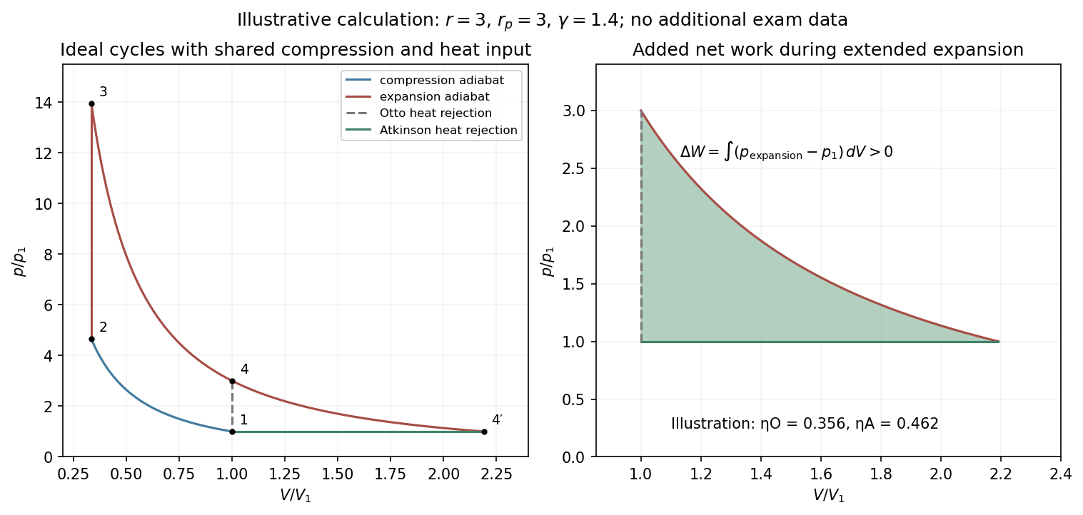
Original ideal-gas cycle calculation showing the extra expansion work and the matched Otto–Atkinson efficiency comparison
. Details. 
For a simple compressible one-component equilibrium system, the fundamental thermodynamic relation isThe internal energy has natural variables : its derivatives give , and chemical potential . The natural variables of a thermodynamic potential identify the independent arguments whose conjugates appear directly in a potential's differential. A Legendre transform exchanges a variable for its conjugate, giving potentials suited to different controlled conditions:
| potential | definition | natural variables | differential |
|---|---|---|---|
| internal energy | |||
| enthalpy | |||
| Helmholtz free energy | |||
| Gibbs free energy |
For fixed composition and the appropriate closed-system constraints, equilibrium minimizes at fixed , at fixed , at fixed , or at fixed , with other allowable internal variations understood. Enthalpy is useful for constant-pressure heat exchange with only pressure–volume work. Helmholtz free energy is suited to fixed-temperature, fixed-volume systems, and Gibbs free energy to fixed-temperature, fixed-pressure phase or chemical equilibrium. Coexisting phases of one substance have equal chemical potentials.
Where a potential is twice continuously differentiable, equality of mixed derivatives gives Maxwell relations. At fixed , the four usual forms areThe fixed subscripts and signs follow from the chosen natural variables. Derivatives through a nonsmooth phase boundary require separate phase descriptions rather than automatic use of the smooth single-phase formulas.
As an application, the Helmholtz relation turns pressure data into an isothermal entropy change. For an ideal gas, , givingCombining the same relation with yields , which vanishes for an ideal gas and reveals attractive-energy effects for a van der Waals gas. Thermodynamic potentials organize equilibrium constraints, while Maxwell relations convert difficult entropy derivatives into measurable response derivatives.
Articles by others on the same topic
There are currently no matching articles.