Source release: Oxford examination archive, member
FOI-20210708-1 - Data/4319.pdf. The cover dates this examination to 23 June 2014, 9.30–11.00am. All seven questions and their 34 leaf subparts are answered below.For an odd prime , the Legendre symbol isIt depends only on the congruence class of the integer . The values and distinguish a nonzero quadratic residue from a quadratic nonresidue; zero is a separate case.
Euler's criterion states, for an odd prime ,Apply it to . The integer is when and when . Since those signs are distinct modulo an odd prime, the modular congruence determines the actual Legendre symbol:This is the first supplementary law for quadratic reciprocity.
For , the residues are simply , with no reduction needed. Write . A term exceeds exactly when , soIf is congruent to modulo eight, the parity of this count is respectively even, odd, odd, even. Gauss's lemma therefore givesThis proves the second supplementary law for quadratic reciprocity, rather than merely applying it.
Because is odd, must be odd. Every odd square is modulo eight. If is even, is zero modulo eight; if is odd, it is two modulo eight. ThusMore precisely, the first case has even and the second has odd . These are necessary conditions on the congruence class, as requested; the elementary calculation alone does not prove their sufficiency.
Equivalently, reduction modulo makes a quadratic residue: cannot divide , since that would also force and hence . The two supplementary laws and multiplicativity of the Legendre symbol give the same two allowed classes.
Writing , the second condition becomes . Writing , its second condition becomes . Consequentlygives an infinite set of positive integer solutions. Conversely these are the positive solutions in the indicated congruence classes, by the Chinese remainder theorem.
Choose any pair from part (i), and put . The divisibilities of the exponents makepositive integers. Their powers areThus , with all three powers nonzero and distinct. For example, take , for every nonnegative integer . Then strictly increases, giving infinitely many distinct solutions. The construction uses modular congruences to turn the elementary identity into three prescribed perfect powers.
A simple group is a nontrivial group whose only normal subgroups are itself and the trivial subgroup.
A composition series is a chain in which each is a normal subgroup of and each quotient group is simple and nontrivial. Its length is , and these quotients are its composition factors. The individual terms need not all be normal in .
A solvable group is a group whose derived series reaches the trivial group: starting with , define . For finite groups this is equivalent to having a composition series whose factors are all cyclic groups of prime order.
Let be the given length-two composition series. Thus and are simple groups. Let be any proper nontrivial normal subgroup of , such as the penultimate term of another composition series.
If , its two factors are already the given ones. Suppose . Since is normal in the simple group , it is either or . The latter would mean , but then would be a proper nontrivial normal subgroup of , impossible. Thus .
Also cannot be contained in , since it would then be a nontrivial normal subgroup of distinct from . The product is a normal subgroup of , strictly containing . Simplicity of therefore forces . The second isomorphism theorem for groups givesIn particular is simple. Every other composition series has such an as its last proper term, and no nontrivial refinement inside a simple is possible. Hence every composition series has length two.
The general Jordan–Hölder theorem states that any two composition series of a finite group have the same length and the same composition factors up to group isomorphism and permutation. The argument above proves both assertions in this length-two case: another series either uses itself or has factors isomorphic to the original pair in the opposite order. No general uniqueness theorem was used to prove this special case.
Factor the group order as . The Sylow theorems say that the number of Sylow subgroups for the prime seven divides and is congruent to one modulo seven. Among , only one qualifies. Thus there is a unique normal subgroup of order .
Every group of prime-square order is Abelian. Indeed its center of a group is nontrivial, and a cyclic quotient by the center of a group forces the whole group to be abelian. Consequently is either or , and in either case it has two composition factors, both .
It remains to consider , of order twelve. Its number of Sylow subgroups for the prime three is either one or four:
- If it is one, the normal order-three subgroup has factor , and the remaining quotient has order four. An order-four group is abelian and has two factors .
- If it is four, these order-three subgroups have disjoint nonidentity elements and account for eight elements. Any Sylow subgroup for the prime two, of order four, must consist of the four remaining elements, since its nonidentity elements have power-of-two orders. It is therefore unique and normal. Its two factors are , and the quotient has order three, giving .
Lift the composition series of to using the subgroup correspondence theorem, and join it to a composition series inside . This givesas the multiset of composition factors. The Jordan–Hölder theorem makes this independent of the chosen series. In particular every group of order is a solvable group, with composition length five; that is a statement about composition length, not necessarily its derived length.
The required general linear position condition is that every of the representing vectors are linearly independent. Such an ordered configuration is a projective frame.
Choose representatives of the first projective points; they form a basis. Write a representative of the last point as . Every is nonzero: otherwise the last point together with the other basis points would fail the independence condition. Rescale the basis representatives to , so that .
Do the same for the target configuration, obtaining representatives with . The unique linear map sending the basis to is invertible and also sends to . Its induced projective transformation sends every point to its prescribed partner. Thus any two ordered projective frames are projectively equivalent.
A projective quadric is the zero locus of a nonzero homogeneous quadratic polynomial , with symmetric over a field of characteristic different from two. A projective point on it is singular when all first partial derivatives vanish. Since , the quadric is nonsingular exactly when is invertible.
Over the complex numbers, a nonzero quadratic form in three variables can be diagonalized by an invertible change of basis. Its rank classifies a projective conic:
- Rank three gives a nonsingular conic.
- Rank two gives two distinct projective lines, since the reduced form factors as . Their intersection is the singular point.
- Rank one gives a double projective line, defined by a squared linear form. The gradient vanishes along that line.
The zero polynomial is excluded from the definition of a conic. Thus these last two cases are precisely the singular conics.
Use part (a) to put the four projective points atA quadratic polynomial vanishing at the first three has no square terms, and vanishing at the fourth givesThese form a two-dimensional vector space. Choose the two membersTheir coefficient triples are independent and both satisfy the relation. Their symmetric bilinear form matrices are of the formFor and , both determinants are , so both selected conics are nonsingular. Any coefficient triple with zero sum is uniquely a linear combination of these two. Hence every conic through the four points has matrixUndoing the projective transformation carries the entire family back to the original four points, preserving nonsingularity. This is a pencil of conics through four points.
For the explicit basis in part (c), has coefficients . ThusAt these values the conics factor, up to nonzero constants, asGeometrically these are exactly the three pairings of the four base points into two pairs, with a projective line joining each pair. No double line can contain four points in general linear position.
The numerical parameter values depend on the selected basis, but the three distinct singular members do not. Another pair of independent nonsingular basis conics gives an invertible projective change of pencil parameter. Its parameter infinity is nonsingular because the second basis form is nonsingular. Therefore all three singular members again occur at three distinct finite values of . This proves the claimed count for any such basis.
The Fréchet derivative at a point is the unique linear map such thatThe error divided by tends to zero as . In standard coordinates this linear map is represented by the Jacobian matrix, but the derivative itself is the map acting on increments, not merely a list of directional rates.
Factor . The determinant expansion near the identity isthe linear terms in the permutation formula come from choosing one diagonal increment and all remaining identity entries. ThereforeThe required Fréchet derivative is the linear functionalThe quadratic remainder proves full differentiability, rather than only the existence of each directional derivative. This is the derivative of the determinant.
The regular level set theorem says that a map with surjective derivative at every point of has a zero set that is an embedded submanifold of dimension . At each point of that zero set,For a smooth map the submanifold is smooth. The full-rank hypothesis is essential for this kernel description when using a particular defining map.
Apply the regular level set theorem to on the -dimensional vector space of real matrices. At a point with determinant one, part (b) gives . Choosing gives , so this derivative is surjective.
Hence the special linear group is a smooth submanifold of dimension . At the identity,This is the special linear Lie algebra. When , the group is a single point and the tangent space is zero, consistent with the same formula.
Use the six-dimensional vector space of real symmetric matrices as the target, rather than all nine matrix entries independently. DefineIts derivative isThe given is symmetric with . Every is invertible, since taking determinants of gives . For any symmetric target , chooseThen , and its transpose is also . Thus and the derivative is surjective at every point of .
The regular level set theorem now givesIt also proves smooth embeddedness in the entire ambient vector space of matrices. The target symmetry is what gives the correct codimension.
The tangent space at the identity is the kernel of a linear map from part (i):This says precisely that is skew-symmetric. Since , multiplication by identifies this tangent space with the three-dimensional space of skew-symmetric matrices. In entries it isSubstitution verifies the equation directly and displays its three independent parameters.
Take a smooth variation . Differentiating the functional at zero gives the first variationIntegrate the second term once and the third term twice by integration by parts:Choose variations supported away from the endpoints. Stationarity and the fundamental lemma of the calculus of variations forceThis is the Euler-Lagrange equation for a second-derivative functional. With the interior equation imposed, the remaining boundary expression must vanish for every admissible variation.
At each endpoint, a freely varying value requires , and a freely varying slope requires . A fixed value or slope instead makes its corresponding variation zero and supplies no natural condition for that variable. These are the natural boundary conditions for second-derivative functionals, with the value and slope variations treated independently.
Here , , and . The Euler-Lagrange equation for a second-derivative functional is thereforeWrite . After imposing the clamped conditions at zero, the general solution isFree right endpoint. Both endpoint variations are free, so the natural boundary conditions for second-derivative functionals give . Since and , they give , . HenceRight endpoint with fixed height and free slope. Now is imposed, while the free slope gives . These equations yield and , soBoth endpoints clamped. The right conditions are , giving , . ThusEach formula has fourth derivative and satisfies all four boundary conditions of its case. The three endpoint choices therefore change the integration constants, not the interior differential equation.
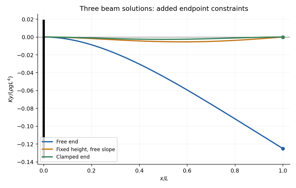
Elastic beam deflections under three right-end boundary conditions
. Original dimensionless plots of the three quartic solutions. Each beam is clamped horizontally at the left. Requiring the right height, then the right slope as well, progressively restricts the admissible deflections. Details.The sets of admissible functions are nested:All impose the same left conditions; the right height adds a restriction, and the right slope adds another. Minimizing the same functional over a smaller set cannot lower its minimum. ThereforeThe doubly clamped beam has the greatest minimum energy, and the free-ended beam the smallest. No energy integrals are needed. In fact the inequalities are strict: the positive quadratic bending term makes the minimizer unique on the left-clamped space, and the three solutions in part (b) are different. The relevant principle is monotonicity of a constrained minimum under added constraints.
A Hamilton cycle is a cycle visiting every vertex of a finite graph exactly once before returning to its starting point. A Hamilton path is a path visiting every vertex exactly once, with no requirement to return or to have its endpoints adjacent. Both conditions concern visiting vertices, rather than traversing every edge.
Let be a longest path in the finite simple graph. Every neighbor of either endpoint lies on this path, since an outside neighbor would extend it. Define two subsets of :Their sizes are and . The degree hypothesis gives , but there are only possible indices. Hence some belongs to both. The edges at that index close a cycle through every vertex of the path:The graph is connected: any component has at least vertices by the minimum degree, so two components would exceed vertices. If , connectedness gives an edge from this cycle to an outside vertex. Starting at that vertex and traversing the cycle without its closing edge gives a path with vertices, a contradiction.
Thus and the cycle is a Hamilton cycle, proving Dirac's theorem. The overlap-of-indices argument is why the degree threshold is half the number of vertices.
Take the complete bipartite graph . Its seven vertices have degrees four on one side and three on the other. Deleting any two vertices leaves at least one vertex on each side, so the remaining complete bipartite graph is connected.
Every cycle in a bipartite graph alternates between its two parts, using equal numbers of vertices from each. A Hamilton cycle here would have to use three vertices from one part and four from the other, which is impossible. Thus three-vertex connectivity and minimum degree three do not suffice for Hamiltonicity in this seven-vertex example.
The Ramsey number is the least positive integer such that every red-blue coloring of the edges of has a red or a blue . Equivalently, every -vertex graph has a clique of size or an independent set of size .
For , either there is a blue edge or every edge is red, producing the red . Conversely an entirely red has neither a red nor a blue edge. Therefore
Put , and consider any coloring of . Choose a vertex . Among its neighbors, either at least are joined to it by red edges, or at least by blue edges.
In the red case, the induced complete graph on those neighbors contains either a red , which joins with to make a red , or a blue . The blue case similarly gives a red or a blue which extends with to a blue . Hence every coloring has the required configuration, andThis is the Ramsey number recursion.
Fix . It has five incident edges, so three of them have the same color by the pigeonhole principle. Suppose they are red, with other endpoints . Any existing edge among must be blue, or it would complete a red triangle with .
If all three edges among existed, they would therefore form a blue triangle. Thus their triple must contain the unique missing edge . In particular, both and belong to the three red neighbors, so and are both red. The identical argument works if the chosen three edges are blue.
Therefore and have the same color for every . The missing edge is crucial: it is the only way the monochromatic neighbor triangle can fail to be present.
Use the Minkowski metric with signature and write , . Future-pointing timelike means and . Thusso is again future-pointing timelike.
Let and . In a Lorentz frame where , the future-pointing vector has . Consequently , with equality exactly when has no spatial component in that frame. HenceTaking positive square roots provesEquality holds exactly when are positive scalar multiples of each other. This is the reverse triangle inequality for future timelike vectors, not the Euclidean triangle inequality.
Take spacetime coordinates . Differentiating the initial segment gives the four-velocityThe identity gives , and . The proper time element therefore satisfies , with the future orientation selecting . Thus is proper time along this path.
Since is proper time, the four-acceleration isIts Minkowski norm squared is , so the invariant magnitude of proper acceleration isThe vector is spacelike, which accounts for the minus sign under the square root.
Differentiate each segment and express the four-velocity using a continuous rapidity:At both rapidities are ; at both are . Hence the four-velocity is continuous at both junctions. This expression also gives everywhere, so the parameter remains proper time on the later segments.
Away from the junctions,with successively . The rapidity is continuous but its slope reverses. Thus the four-acceleration has a finite jump to its negative at each junction, while its magnitude stays on either side. There is no velocity jump; the idealized path is continuously differentiable but not twice differentiable at the switching events.
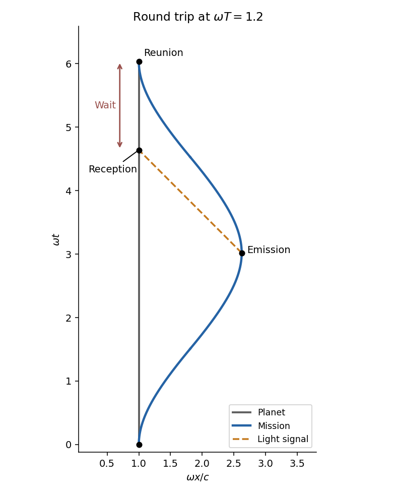
At and , the mission is at the planet's position . The final coordinate time from the last segment isThe planet is at rest in these coordinates, so its proper time elapsed equals this coordinate-time difference. The astronauts' proper time is the parameter interval, . ThereforeFor proper acceleration and , seconds, approximately one year. Thus and . Neglecting in the hyperbolic sine,The clocks compare two different timelike paths between the same departure and reunion events.
Put . At emission, , the middle segment givesThe planet is at , so the inward light signal takes coordinate timeIts arrival time on the planet is therefore . Subtract this from the mission's return time :For large at fixed acceleration this tends to . With the Earth-gravity value above, the wait is approximately two years, despite the millions of planet-years elapsed since departure in part (i).


Articles by others on the same topic
There are currently no matching articles.