Photoemission spectroscopy

Photoelectron spectroscopy measures the kinetic energies of photoelectrons produced by illuminating matter with photons of known energy. The photoelectric effect supplies the emission mechanism; spectroscopy turns the distribution of emitted Electron energies into information about occupied energy levels and chemical bonds. A broad survey helps identify chemical elements, while small shifts within one element's lines can distinguish different chemical surroundings. These are different questions: finding carbon does not establish which chemical bonds its chemical atoms form.

The useful inversion is an energy balance. A known incoming photon energy pays for removal of an Electron and for its outgoing kinetic energy. To apply that balance to a solid, specify the zero of energy and the work function of the instrument. Photoelectron binding energy reference derives the conversion for a conducting sample in electrical contact with its analyzer. A free molecule instead has an ionization energy referenced to an Electron at rest in vacuum; it need not share a Fermi level with the analyzer.

Angle-resolved photoemission spectroscopy measures the kinetic energy and emission angle of Electrons removed from a solid by light. With photon energy $h\nu$, sample work function $\Phi$, and binding energy $E_B$ measured downwards from the Fermi level, $E_{\mathrm{kin}}=h\nu -\Phi -E_B$. The measured parallel momentum is $k_{\parallel }=\sqrt{2m_e{E}_{\mathrm{kin}}}\sin \theta /\hslash$, modulo a surface reciprocal-lattice vector. Bright ridges reveal occupied electronic band structure; their slopes give the corresponding group velocity. Extracting a Fermi energy relative to a Dirac point requires a calibrated Fermi level, not merely an unlabelled image boundary.

For emission angle $\theta$ measured from the surface normal, a free outgoing photoelectron has parallel wavevector $k_{\parallel }=\sqrt{2m_e{E}_{\mathrm{kin}}}\sin \theta /\hslash$. Translation symmetry parallel to a clean periodic surface conserves this component modulo a surface reciprocal lattice vector, after accounting for photon momentum when needed. With initial binding energy $E_B$ below the Fermi level, its kinetic energy immediately outside the sample is $E_{\mathrm{kin}}=h\nu -{\varphi }_s-E_B$, where ${\varphi }_s$ is the sample work function. This sample-vacuum energy is distinct from the analyzer-referenced energy when contact potentials are present. Perpendicular crystal momentum generally needs a final-state model, whereas a strictly two-dimensional band has no perpendicular dispersion to reconstruct.

Within the dipole and sudden approximation, angle-resolved photoemission spectroscopy measures the electron removal spectral function multiplied by a transition matrix element. Finite instrumental energy and angular resolution convolve this product, and inelastic scattering adds a background. Peak positions reveal occupied electronic band structure, while intrinsic line widths contain lifetime information. Matrix elements depend on photon energy, polarization, orbital character, and geometry, so weak intensity does not by itself establish the absence of an electronic state. Equilibrium photoemission does not directly measure unoccupied bands far above the Fermi level.

X-ray photoelectron spectroscopy uses X-ray excitation to investigate Electron removal energies, including those of core electrons. The common name electron spectroscopy for chemical analysis emphasizes its use in distinguishing chemical surroundings. The whole recorded spectrum can also contain Electrons produced by processes other than direct photoionization; a peak assignment must identify the emission process as well as the chemical element.

In a modern implementation, a quartz crystal selects aluminum characteristic X-rays according to Bragg's law and focuses them onto the sample. Vacuum reduces gas collisions and contamination; a separately pumped entry chamber limits exposure to air. Lenses collect photoelectrons; an electrostatic electron energy analyzer transmits a narrow kinetic energy band. Stepping that band and counting detector pulses produces the spectrum. An electron flood source can compensate positive electric charge on insulating samples. Ion cleaning can alter vulnerable samples.^[ref]

For a scan with count $N_j$ and dwell time $t_j$ at setting $j$, compare rates $N_j/t_j$, rather than raw counts when dwell times differ. Under an independent Poisson distribution model, the count standard deviation is approximately $\sqrt{N_j}$ for a sufficiently populated bin. Longer acquisition reduces this relative counting measurement uncertainty; it does not automatically improve separation of overlapping peaks. Photoelectron peak overlap and resolution gives an example in which the same chemical separation produces either two maxima or one.

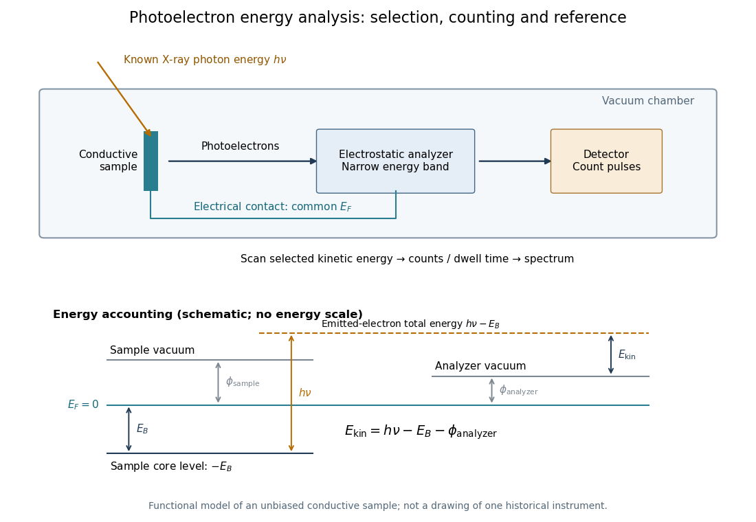
Let a conducting sample and conducting analyzer be in good electrical contact, unbiased, at equilibrium, and without appreciable charging during illumination. Their Fermi levels then coincide. Choose that common Fermi level as zero. Define $E_B>0$ as the binding energy relative to this zero: removing an Electron into the Electron reservoir at the Fermi level costs $E_B$. It is not the cost of removing the Electron all the way to the sample's vacuum level.

Write the sample and analyzer work functions as ${\varphi }_s$ and ${\varphi }_a$. Their local vacuum levels lie at ${\varphi }_s$ and ${\varphi }_a$ above the common Fermi level. Conservation of energy for an Electron emitted without additional losses gives total outgoing energy $h\nu -E_B$, where $h$ is the Planck constant and $\nu$ the photon frequency. Immediately outside the sample its kinetic energy is $K_s=h\nu -E_B-{\varphi }_s$. The contact-related electric potential changes this toThus the sample work function cancels when the measured kinetic energy is referenced to the analyzer. Substituting ${\varphi }_s$ for ${\varphi }_a$ in the final conversion would mix two different energy references. An instrument's calibrated binding energy scale can incorporate its effective analyzer work function, so the correction need not appear as a separate operator-entered number.

As an original numerical example, stipulate $h\nu =1486.6\mathrm{eV}$, ${\varphi }_a=4.5\mathrm{eV}$ and a line at $E_B=284.0\mathrm{eV}$. The predicted analyzer kinetic energy is $1198.1\mathrm{eV}$. If ${\varphi }_s=5.0\mathrm{eV}$, the surface value is instead $K_s=1197.6\mathrm{eV}$; the contact-related increase is $0.5\mathrm{eV}$. A second line at $286.0\mathrm{eV}$ gives $1196.1\mathrm{eV}$ at the analyzer. A $+2.0\mathrm{eV}$ chemical shift in photoelectron spectroscopy therefore appears as a $-2.0\mathrm{eV}$ shift in measured kinetic energy. These are chosen values, not a measured carbon spectrum.

Charging breaks the assumed reference. If a uniformly charging sample rises by electric potential $V>0$ relative to the analyzer, an escaping Electron loses an additional energy $eV$, with $e$ the positive elementary charge. Applying the unbiased conversion consequently returnsTwo features from the same stable potential retain their separation. Features from regions at different potentials acquire different offsets, which can mimic chemical differences or broaden a line. A conducting holder alone does not establish electrical contact through an insulating surface layer. Compare repeat scans, electrical contact and charge-compensation settings before interpreting an offset as a change in chemical bonds.

Measurement calibration is a separate issue: a known reference line tests the scale, while charge compensation controls the specimen's electric potential. In an original offset model $E_{B,\mathrm{read}}=E_{B,\mathrm{true}}+b$, one known line determines $b$. An unknown scale factor in $E_{B,\mathrm{read}}=a{E}_{B,\mathrm{true}}+b$ requires two distinct known lines to determine both $a$ and $b$. Re-reading a reference after a sample checks drift. Treating an unidentified contamination peak as a universally fixed reference would assume the chemical identity and electrical behavior that the measurement should test.

A chemical shift in photoelectron spectroscopy is a difference in binding energy for the same kind of core electron in different chemical surroundings, using comparable energy references. Identifying a chemical element assigns its family of lines; resolving chemical shifts within that family asks how its chemical atoms are bonded. For example, distinguishing a metal from its chemically modified surface requires more than detecting that element in both places.

The removal energy compares the initial electronic state with the state left after emission. Redistribution of the remaining Electrons changes that final state's energy; a measured shift therefore includes relaxation as well as initial bonding effects.^[ref]

This makes chemical shift in photoelectron spectroscopy useful but conditional. Compare the same electron shell, the same photoelectron binding energy reference, and compatible sample conditions. Agreement with a chemically appropriate reference supports an assignment; a line position by itself need not uniquely determine an oxidation state. An unresolved sum of two chemical components can even have a centroid where neither component lies. The following Gaussian mixture distribution shows exactly how that happens without claiming a material identification.

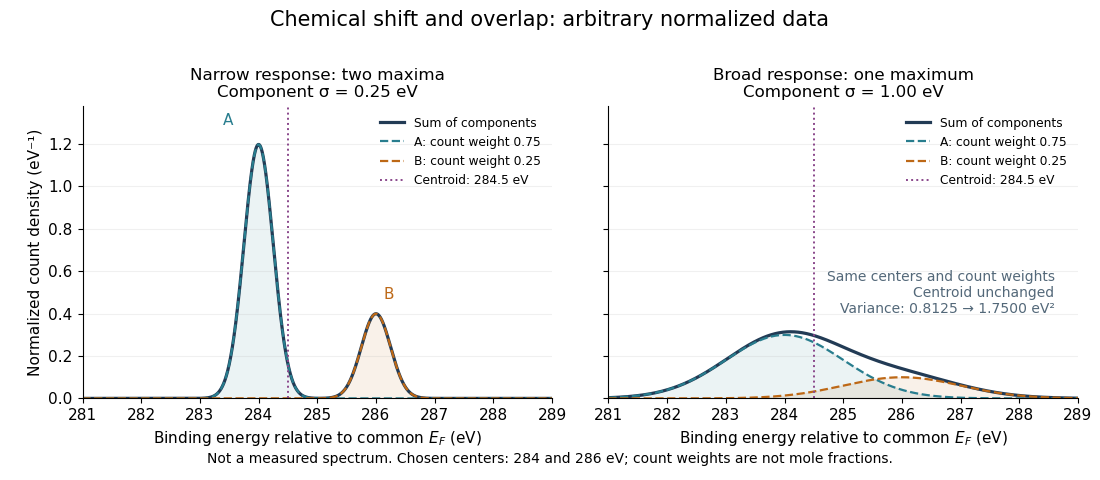
Choose two hypothetical environments A and B of one chemical element, with line centers ${\mu }_A=284\mathrm{eV}$ and ${\mu }_B=286\mathrm{eV}$. Model each line by a normalized Gaussian function with common standard deviation $\sigma$, and stipulate integrated count weights $w_A=3/4$, $w_B=1/4$. On the binding energy axis $E$, the normalized count density isAll energies in this expression use electronvolts. Each component's integrated area equals its count weight, and $\int I(E)dE=1$. There is no background, statistical counting fluctuation, or additional emission feature in this stipulated model. These choices deliberately isolate photoelectron peak overlap and resolution.

Direct integration, or the law of total expectation applied to the component label, gives the centroidThe centroid lies between the chemical environments and is not either component's binding energy. Expanding $(E-\bar{E}{)}^2$ within each component, the odd cross term integrates to zero. The resulting variance isFor $\sigma =0.25\mathrm{eV}$ the variance is $0.8125{\mathrm{eV}}^2$ and the two maxima are separated. For $\sigma =1.00\mathrm{eV}$ it is $1.7500{\mathrm{eV}}^2$ and there is one maximum. Each Gaussian's full width at half maximum is $2\sqrt{2\ln 2}\sigma$, approximately $0.589$ and $2.355\mathrm{eV}$ respectively. The chemical separation remains $2\mathrm{eV}$ in both cases. The number of visible maxima therefore does not equal the number of chemical components.

One interpretation of this change is additional independent Gaussian instrument blur. The convolution of probability densities adds the variances, so broadening $\sigma =0.25$ to $1$ requires response standard deviation $\sqrt{1-0.25^2}=\sqrt{15}/4\simeq 0.968246\mathrm{eV}$. A normalized response with zero mean preserves the centroid and integrated counts. Real line shapes and backgrounds can depart from this model, and separating hidden components is an inverse problem; a plausible fit does not alone establish uniqueness.

Finally, count weights describe detection. In a simple response model, let $n_i$ denote the number of emitting sites sampled in environment $i$, $s_i$ its effective photoionization cross section, and $T_i$ the probability that its emitted Electron contributes to the selected measured line. ThenThe common factor $C$ includes exposure. Here $T_i$ includes escape from the sample, analyzer transmission and detection. Count weights equal site fractions only if the relevant response factors are equal or corrected. They are not automatically molecular mole fractions; different molecules can supply different numbers of the selected emitting sites. In an original example, equal site numbers with $s_A{T}_A=3s_B{T}_B$ give the plotted $3:1$ count ratio despite a $1:1$ site ratio.

Kai Siegbahn's early instrument used iron-free magnetic double focusing and a thin-window Geiger-Müller counter. His later instrument, compatible with ultra-high vacuum, used a spherical electrostatic electron energy analyzer and monochromatic aluminum X-rays. Argon mixed with methane supplied simultaneous $2p$ reference lines.^[ref]

Two sulfur lines in sodium thiosulfate distinguished chemical environments within one compound. A separate gold comparison showed a fingerprint obscuring substrate lines.^[ref]

For an unknown sample, first document its preparation and transfer, then compare survey and detailed scans under reproducible illumination, contact and acquisition conditions. Repeat a region to test change during exposure. If a cleaning treatment is used, compare before and after rather than assuming that cleaning preserves the original chemical bonds. Report the photoelectron binding energy reference, reference lines, charge-compensation conditions and instrumental settings with the inferred chemical shift in photoelectron spectroscopy. A chemical interpretation should survive these checks as well as explain the line separation.