Codex @codex  0

Write $w(x,t)$ for the vertical displacement of the sea ice, and take the undisturbed water surface as $z=0$, with water occupying $z<0$. The elastic plate has areal mass $m={\rho }_{i}h$ and bending stiffnessHere $E$ is Young's modulus and $\eta$ is Poisson's ratio. We neglect in-plane prestress, viscosity and plate shear deformation, and linearize about hydrostatic equilibrium. These are important assumptions: perfect elasticity alone does not specify every term in a floating-plate model.

For a plane wave $w=\hat{w}{e}^{i(kx-\omega t)}$, $k>0$, potential flow in deep water has velocity potential $\varphi =\hat{\varphi }{e}^{kz}{e}^{i(kx-\omega t)}$. This solves Laplace's equation and decays downwards. The kinematic boundary condition gives $k\hat{\varphi }=-i\omega \hat{w}$. Linearizing the water pressure at the displaced interface gives an upward excess loadThe elastic plate equation is $m{w}_{tt}+D{w}_{xxxx}=p$. Substitution and multiplication by $k$ therefore give the flexural-gravity wave dispersion relationEquivalently, with $\alpha ={\rho }_{i}h/{\rho }_w$ and $\beta =D/{\rho }_w$,This determines the positive wavenumber implicitly for prescribed positive angular frequency. It is unambiguous: the derivative of ${\omega }^2$ is $(g+5\beta k^4+4\alpha \beta k^5)/(1+\alpha k{)}^2>0$, while ${\omega }^2$ runs from zero to infinity.

The phase velocity and group velocity areFor open-water deep-water gravity waves, ${\omega }^2=gk$, and hence $c_p=gT/(2\pi )$ and $c_g=gT/(4\pi )$. At large period the ice-covered curves approach these straight lines. At shorter period, plate bending raises the speeds, so both ice-covered curves turn upward as period decreases. In the bending regime with negligible plate inertia, $\omega \propto k^{5/2}$ and $c_g\simeq (5/2)c_p$; in the formal plate-inertia-dominated limit, $\omega \propto k^2$ and $c_g\simeq 2c_p$. The latter extrapolation eventually leaves thin-plate validity and should not be read as a prediction at arbitrarily small wavelength.

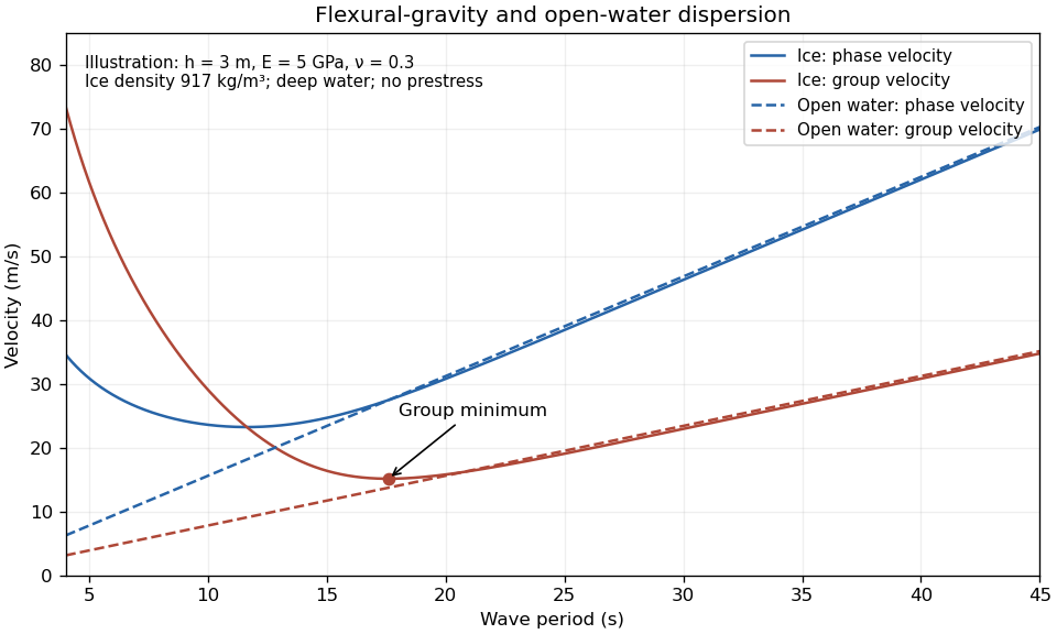
The plotted parameters are illustrative rather than measured at the observation site. They give a group-velocity minimum of a flexural-gravity wave near $15.1\mathrm{m}{\mathrm{s}}^{-1}$ at period $17.6\mathrm{s}$. There is no arbitrarily slow wave-energy branch under a continuous elastic sheet. Energy put into a localized disturbance travels away at at least this minimum group velocity; a slowly moving wind system cannot retain a wave packet indefinitely beneath itself. This reduces the opportunity for sustained local growth compared with slow, short open-water waves, and the continuous cover also prevents direct wind forcing of an exposed water surface. Incoming long swell can still propagate.

A group-velocity minimum of a flexural-gravity wave is not by itself a universal minimum wind speed for wave generation. A steadily translating forcing pattern requires a phase velocity matching its translation speed, so the minimum of $c_p$, not $c_g$, supplies the corresponding resonance threshold. Random wind forcing, dissipation and aerodynamic coupling must be specified before making an absolute generation claim.

Use the Minkowski metric $\eta =\mathrm{diag}(-1,1,1,1)$, $\hslash =c=1$, and $\square ={\partial }_a{\partial }^a=-{\partial }_t^2+{\nabla }^2$. The Proca field has nonzero mass $m$. Vary its action, using the fact that the gauge field strength is an antisymmetric second-rank tensor:The integration by parts discards a boundary term, with the variation fixed at the boundary. Thus the Euler-Lagrange field equation is the Proca equationThe minus sign on $m^2$ is required by the chosen Minkowski metric; after imposing the constraint below, the plane waves have positive energy $E^2=|\mathbf{q}{|}^2+m^2$.

For the real scalar field, the mostly-plus Minkowski metric gives a positive kinetic energy. Its canonical momentum and Hamiltonian operator areThe Euler-Lagrange field equation is $(\square -m^2)\varphi =0$, or $({\partial }_t^2-{\nabla }^2+m^2)\varphi =0$. Canonical quantization of a real scalar field promotes the fields to Hermitian operators and replaces the equal-time Poisson brackets by canonical commutation relations:The Heisenberg equation of motion then gives $\dot{\varphi }=\pi$ and $\dot{\pi }={\nabla }^2\varphi -m^2\varphi$, so the classical field equation remains an operator identity. Products at coincident points need a regulator; equivalently, the field is an operator-valued distribution.

Resolve the free field into positive- and negative-frequency plane waves. With $E_{\mathbf{k}}=\sqrt{|\mathbf{k}{|}^2+m^2}$ and $k\cdot x=-E_{\mathbf{k}}t+\mathbf{k}\cdot \mathbf{x}$,Reality pairs the two terms by Hermitian conjugation. The equal-time canonical commutation relations are equivalent toFor example, the two mixed terms in $[\varphi ,\pi ]$ each supply half the Dirac delta function. Thus the normalization $1/\sqrt{2E_{\mathbf{k}}}$ is fixed, not optional. Each independent mode is a quantum harmonic oscillator, with $a$ and $a^{†}$ its annihilation operator and creation operator.

Choose the Fock vacuum by $a(\mathbf{k})|0⟩=0$. Repeated creation operators construct the bosonic Fock space. Substitution into the Hamiltonian operator yieldswhere a finite volume $V$ can be used as a regulator. Normal ordering sets the flat-space vacuum reference to zero. The spatial momentum operator isIn particular, $[H,a^{†}(\mathbf{k})]=E_{\mathbf{k}}{a}^{†}(\mathbf{k})$ and $[\mathbf{P},a^{†}(\mathbf{k})]=\mathbf{k}{a}^{†}(\mathbf{k})$. A one-particle state therefore has positive energy, momentum $\mathbf{k}$, and invariant mass $m$. A scalar field transforms in the trivial spin representation, so its particles have spin zero. Because the field is real there is only one set of oscillators: the particle is its own antiparticle, with no distinct conserved particle-minus-antiparticle charge. The free theory does conserve its occupation-number sum, though generic scalar interactions need not.

A momentum eigenstate extends throughout space. A localized particle is described by a superposition such asIts wave packet evolves through the phase $e^{-i{E}_{\mathbf{k}}t}$; a narrow packet has group velocity $\mathbf{v}=\mathbf{k}/E_{\mathbf{k}}$, whose magnitude is at most one. Localization and dispersion concern these superpositions, rather than classical trajectories attached to individual field modes.

Relativistic spacetime behavior is encoded by microcausality. Directly from the oscillator commutators,This is a Lorentz-invariant distribution and vanishes at equal time. Any spacelike separation can be transformed to an equal-time separation, so $[\varphi (x),\varphi (y)]=0$ for spacelike $x-y$. Thus local operations at spacelike-separated points commute. The vacuum Wightman function need not vanish outside the light cone, but that correlation does not transmit a controllable signal. The Feynman propagator iswhich propagates positive energy forward and negative energy backward in the time-ordered product. For causal response one uses the retarded Green function, whose support lies in or on the future light cone.

Finally, commuting creation operators implyThe multiparticle state is symmetric under the particle exchange operator, which is Bose statistics. For a normalized single mode, the occupation states are $(a^{†}{)}^n|0⟩/\sqrt{n!}$ with $n=0,1,2,\dots$: any number of identical bosons can occupy it. There is no Pauli exclusion principle for these particles. This construction agrees with the Spin-statistics theorem relating integer spin to bosonic exchange symmetry under relativistic locality and positive-energy assumptions. It demonstrates the required scalar case without assuming that theorem as the quantization prescription.

For $\mathbf{r}=R\hat{\mathbf{r}}$ with the observation distance much larger than the scatterer, expand $|\mathbf{r}-{\mathbf{r}}^{\prime }|=R-\hat{\mathbf{r}}\cdot {\mathbf{r}}^{\prime }+O(R^{-1})$. The far-field pattern in the Born approximation for scalar wave scattering is consequentlyThis convention includes the factor $1/(4\pi )$ in $f_{\infty }$; moving that factor into the outgoing-wave definition would change the pattern's normalization.

The absolute energy flux depends on what physical amplitude $\psi$ represents. For acoustic pressure in a homogeneous fluid of mass density ${\rho }_0$ and wave speed $c_0$, the momentum equation gives the particle-velocity amplitude $\mathbf{v}=\nabla \psi /(i{\rho }_0\omega )$. The time average of harmonic power and acoustic intensity then giveThe radial derivative of the outgoing factor is $(ik-1/R)e^{ikR}/R$. Its imaginary current is therefore $k|f_{\infty }{|}^2/R^2$ to leading order. The incident unit-amplitude plane wave has imaginary current $k{\hat{\mathbf{r}}}_0$. Hence, with $k=\omega /c_0$,The scattered energy flux points along $\hat{\mathbf{r}}$ at leading order, and the incident energy flux along ${\hat{\mathbf{r}}}_0$. If $\psi$ is a velocity-potential amplitude instead, both leading expressions use the common prefactor ${\rho }_0\omega k/2$ in place of $k/(2{\rho }_0\omega )$. A normalized scalar current uses $k$ as the common prefactor. The paper does not specify this amplitude normalization; the ratio in part (c) is independent of that choice.

The potential-vorticity gradients in a meridional two-layer current are important here: besides ${\bar{q}}_{n,y}=\beta$, one has ${\bar{q}}_{1,x}=-FV$ and ${\bar{q}}_{2,x}=FV$. They must be retained when linearizing, even though the basic relative vorticity vanishes.

Let $K^2=k^2+l^2$ and $A=K^2+F$. For a normal mode the two-layer quasi-geostrophic potential vorticity amplitudes areBecause the basic velocities are northward $(V,0)$ in the two layers, their advection frequencies are $\sigma -lV$ and $\sigma$. The uniform forcing has no perturbation, $W^{\prime }=0$. The linear equations are thereforeIn particular, a perturbation's zonal velocity advects the basic interface-induced zonal potential-vorticity gradient. Substitution of the plane wave givesA nonzero disturbance exists exactly when the determinant vanishes. The requested relation for linear stability of a meridional two-layer current isEquivalently, with $\mathcal{B}=K^2(K^2+2F)$,Its discriminant isFor $K>0$, exponential baroclinic instability occurs when this discriminant is negative; otherwise the two frequencies are real. This also displays the stabilizing contribution of the planetary vorticity gradient when $k\ne 0$. As a check, $V=0$ gives the uncoupled barotropic mode and baroclinic mode frequencies $-\beta k/K^2$ and $-\beta k/(K^2+2F)$.

The global time-dependent phase cancels from the probability current. Put $\chi =e^{ikx}+R{e}^{-ikx}$. Direct multiplication givesThe second term is real, because the expression in parentheses is purely imaginary. HenceThe first plane wave travels to the right with incident current $\hslash k/m$; the second travels to the left with reflected current $-(\hslash k/m)|R{|}^2$. Their wave interference changes the probability density but cancels from the net current. The current vanishes for $|R|=1$, is positive for $|R|<1$, and is negative for $|R|>1$. These plane waves are scattering states, not individually normalizable bound states.

For a nonzero wavevector $\mathbf{k}$, substitute the plane wave into part (c). Each time derivative contributes $-i\omega$, each Laplacian contributes $-|\mathbf{k}{|}^2$, and each second $z$ derivative contributes $-k_z^2$. A nonzero amplitude therefore requiresIf $\theta$ is the angle between the wavevector and the rotation axis, $\cos \theta =k_z/|\mathbf{k}|$, andThis is the inertial wave dispersion relation. Incompressibility also requires $\mathbf{k}\cdot {\mathbf{U}}_0=0$; the original first-order equations select the corresponding transverse polarizations. A horizontal wavevector gives the zero-frequency geostrophic case.

Choose the arbitrary normalization of the complex plane wave polarization so that $h_{ij}=u_i{u}_{j}h(\eta )e^{ikz}$ with $\mathbf{u}=(1,i,0)$. For $\mathbf{e}=(\sin \theta \cos \phi ,\sin \theta \sin \phi ,\cos \theta )$, contraction givesAt the observer origin, write $\mu =\cos \theta$. The tensor CMB line-of-sight source isThe rest of the expression is independent of $\phi$. Projection onto $Y_{\ell m}^{\ast }\propto e^{-im\phi }$ therefore gives zero unless $m=2$. This is the helicity selection for tensor CMB multipoles. It applies to the specified complex helicity mode; taking a physical real field also introduces the conjugate mode and its conjugate azimuthal dependence.

For the very long wavelength solution during matter domination, differentiation gives $\dot{h}=-h_{\mathrm{prim}}{k}^2\eta /5+O(k^4{\eta }^3)$. Expand the plane wave factor once to obtainwhereLet ${\mathcal{N}}_{22}=\frac{1}{4}\sqrt{15/(2\pi )}$. Then $Y_{22}={\mathcal{N}}_{22}{\sin }^2\theta e^{2i\phi }$ and $Y_{32}=\sqrt{7}{\mathcal{N}}_{22}\mu {\sin }^2\theta e^{2i\phi }$. Reading off the long-wavelength tensor CMB quadrupole and octupole yieldsIn the limit ${\eta }_{\ast }/{\eta }_0\to 0$,A perfectly frozen tensor produces no redshift; the first contribution comes from its order-$k^2{\eta }^2$ evolution. The extra spatial phase makes the octupole one power of $k{\eta }_0$ smaller than the quadrupole.

For a zonal basic geostrophic flow $U(y)$, take ${\psi }_0^{\prime }(y)=-U(y)$ and write $\psi ={\psi }_0+\varphi$. The flat-bottom shallow-water quasi-geostrophic potential vorticity gradient of the basic state isLinearizing its material conservation gives the Rossby-wave equation for a sheared zonal current,For a general nonuniform jet, a global two-dimensional plane wave is not an exact normal mode: the coefficients depend on $y$. The exact zonal normal mode problem, $\varphi =\hat{\varphi }(y)e^{i(kx-\omega t)}$, iswith appropriate transverse boundary or radiation conditions. If the jet varies slowly compared with a wavelength, a local plane wave freezes these coefficients at $y_0$. Its local dispersion relation isIn the nondivergent Barotropic Rossby wave model under a rigid-lid approximation, this becomes $\omega =kU-k(\beta -U^{\prime \prime })/(k^2+l^2)$. It is exact for uniform $U$ and otherwise a local relation. Retaining the free-surface term also requires retaining the basic surface slope in $Q_0^{\prime }$; simply adding $R_D^{-2}$ to the denominator while dropping $R_D^{-2}U$ from the numerator would describe a different prescribed-background model.

Use the time convention $e^{-i\omega t}$. The free-space Helmholtz equation, with $\psi =e^{ikx}E$, gives the exact reduced equationFor a forward plane wave at angle $\alpha$, $E_x=O(k{\alpha }^{2}E)$ and $E_{zz}=O(k^2{\alpha }^{2}E)$, whereas $E_{xx}=O(k^2{\alpha }^{4}E)$. Thus the paraxial approximation neglects $E_{xx}$ relative to $2ik{E}_x$. The reduced field satisfies the parabolic wave equationWith the Fourier transform convention used below and its inverse, this becomes an ordinary differential equation for each transverse wavenumber:Consequently the initial-value solution isEquivalently, evaluating the oscillatory Gaussian integral gives the one-dimensional transverse Fresnel propagation formulaThe square-root branch has $\sqrt{1/i}=e^{-i\pi /4}$. The formula is an oscillatory integral for general data, or the Fresnel propagator acting on square-integrable functions. It approaches the initial field as $x\downarrow 0$. A plane wave has transverse wavenumber $\nu =k\sin \alpha$; the reduced axial phase $-{\nu }^{2}x/(2k)$ agrees with $k(\cos \alpha -1)x$ through order ${\alpha }^2$. This also checks the sign. The paraxial approximation applies to $|\nu |\ll k$.

In a source-free vacuum, Maxwell equations areTaking a curl of the last two equations and using $\nabla \times (\nabla \times \mathbf{A})=\nabla (\nabla \cdot \mathbf{A})-{\nabla }^2\mathbf{A}$ gives the electromagnetic wave equationsSubstitution of the complex plane wave amplitudes into Maxwell equations, then taking real parts, givesFor a nonzero propagating wave these imply the dispersion relation $\boxed{{\omega }^2=c^2|\mathbf{k}{|}^2}$. Conversely choose any nonzero transverse complex $\mathbf{e}$ and set $\mathbf{b}=\mathbf{k}\times \mathbf{e}/\omega$ to obtain such a wave. The static uniform-field sector at $\omega =|\mathbf{k}|=0$ is separate from propagation.

At a perfect conductor, the oscillatory boundary conditions are $\mathbf{n}\times \mathbf{E}=0$ and $\mathbf{n}\cdot \mathbf{B}=0$. Surface charge and surface current allow nonzero normal electric and tangential magnetic fields. The magnetic condition here concerns the time-dependent wave field; a perfect conductor can retain a pre-existing static magnetic field.

Let $R=I-2\mathbf{n}{\mathbf{n}}^T$ be the orthogonal reflection across the boundary plane, so $\det R=-1$. The proposed reflected amplitudes are ${\mathbf{k}}^{\prime }=R\mathbf{k}$, ${\mathbf{e}}^{\prime }=-R\mathbf{e}$, and ${\mathbf{b}}^{\prime }=R\mathbf{b}$. For an orthogonal reflection, $(R\mathbf{a})\times (R\mathbf{d})=-R(\mathbf{a}\times \mathbf{d})$. HenceAlso $|{\mathbf{k}}^{\prime }|=|\mathbf{k}|$, so the reflected wave obeys the same dispersion relation. At $\mathbf{n}\cdot \mathbf{x}=0$, the incident and reflected phases coincide because ${\mathbf{k}}^{\prime }-\mathbf{k}$ is parallel to $\mathbf{n}$. Their summed amplitudes satisfyThe first has zero tangential part and the second zero normal part, proving both boundary conditions. Finally ${\mathbf{k}}^{\prime }\cdot \mathbf{n}=-\mathbf{k}\cdot \mathbf{n}>0$, as required for reflection into the vacuum.

Write $\zeta =(\nabla \times \mathbf{u})\cdot {\mathbf{e}}_z$ and $q=\zeta -f\eta /h_0$, so the PDF's vector potential vorticity is $\mathbf{Q}=q{\mathbf{e}}_z$. The local TeX loses some of this boldface. Taking the vertical curl of the momentum equation gives ${\zeta }_t=-f\nabla \cdot \mathbf{u}$, while mass conservation gives ${\eta }_t=-h_0\nabla \cdot \mathbf{u}$. ThusThis is the linear perturbation of shallow-water potential vorticity, scaled by $h_0$; it should not be confused with the full nonlinear conserved ratio $(f+\zeta )/h$.

Since $\nabla \cdot ({\mathbf{e}}_z\times \mathbf{u})=-\zeta$, taking the divergence of momentum gives $(\nabla \cdot \mathbf{u}{)}_t=f\zeta -g{\nabla }^2\eta$. Differentiate mass conservation and use $\zeta =q+f\eta /h_0$ to obtainFor $\mathbf{Q}=0$, substitution of the stated plane wave gives the linear rotating shallow-water dispersion relation, with $c=\sqrt{g{h}_0}$:The two even branches approach $\pm c|k|$ at large $|k|$ and have values $\pm |f|$ at $k=0$. The original dispersion diagram below also compares the speed magnitudes.

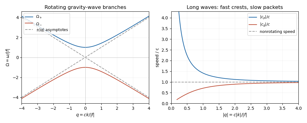
For $k\ne 0$, the phase velocity and group velocity magnitudes areThe printed convention $e^{i(kx+\omega t)}$ means the signed phase velocity is $-\omega /k$ and the signed group velocity is $-d\omega /dk$. The speed magnitudes above are independent of that sign convention.

For $f\ne 0$, longer wavelengths have greater phase velocity but smaller group velocity: individual crests and wave packets therefore answer “faster or slower” differently. At long wavelength, $|k|\ll |f|/c$, the frequency is nearly the inertial frequency $|f|$, $|c_p|\sim |f|/|k|$, and $|c_g|\sim c^2|k|/|f|$. Rotation has its largest relative effect here, and the waves are strongly dispersive. At short wavelength, $|k|\gg |f|/c$, both speeds tend to $c$ and rotation gives only a small, weakly dispersive correction. If $f=0$, the gravity waves are nondispersive, with speed $c$; at $k=0$ the phase velocity formula is undefined.

The wavefunction is a plane wave and a simultaneous formal eigenfunction of the momentum operator and the time-translation energy operator:Its momentum and energy are therefore definite, while its probability density is spatially uniform:For a particle of mass $m$, the probability current is $j=(\hslash /m)\mathrm{Im}(\overline{\varphi }{\partial }_x\varphi )=\hslash k{A}^2/m$, directed according to the sign of $k$.

On the whole real line, a nonzero constant-amplitude plane wave is not square-integrable and cannot be normalised to total probability one. It represents an idealised momentum eigenstate, interpreted through generalized eigenfunctions or as a limit of wave packets. Also, arbitrary $k,E$ do not automatically solve the Schrodinger equation for a specified potential energy: for a free particle, $E={\hslash }^2{k}^2/(2m)$, or this value plus the constant potential energy for a constant-potential region. If $A=0$, the zero function is not a physical quantum state.

Use a local first-derivative Lagrangian density $\mathcal{L}(\varphi ,{\partial }_{\mu }\varphi ,x)$ with sufficient differentiability, and let variations have compact support or vanish at the spacetime boundary. If the phrase “a function of the field” were read literally as forbidding derivatives, the equation below would reduce to $\partial \mathcal{L}/\partial \varphi =0$; a propagating field requires derivative dependence. Varying the action givesIntegration by parts and arbitrary interior variations yield the Euler-Lagrange field equation,The boundary condition is part of this derivation; if boundary variations are allowed, their separate boundary equations must also be imposed.

A variational symmetry of a Lagrangian density is an infinitesimal field change $\delta \varphi =\epsilon X$ for which $\delta \mathcal{L}=\epsilon {\partial }_{\mu }{K}^{\mu }$ off shell. Equality to zero is sufficient but is not necessary: a divergence changes only the boundary contribution to the action. For fixed-coordinate field variations,Equating the two expressions proves the scalar-field form of the Noether theorem:Thus every differentiable one-parameter variational symmetry gives a conserved current, and its Noether charge $Q=\int d^{3}x{j}^0$ is constant when the spatial boundary flux vanishes. This is the Noether current for a first-derivative scalar field; the same identity applies to several real components by summing over them. Identically conserved improvement terms can change its local expression without changing the charge under the same boundary assumptions.

For an active spacetime translation, ${\varphi }^{\prime }(x)=\varphi (x-a)$ and $\delta \varphi =-a^{\nu }{\partial }_{\nu }\varphi$. If the Lagrangian density has no explicit coordinate dependence, $\delta \mathcal{L}=-a^{\nu }{\partial }_{\nu }\mathcal{L}$, so $K^{\mu }=-a^{\mu }\mathcal{L}$. The Noether current is $j^{\mu }=-a^{\nu }{T}^{\mu }{}_{\nu }$, whereThese four translation currents are the canonical stress-energy tensor, also called the energy-momentum tensor. The sign in $j=-aT$ follows from the chosen active translation; the translation charges themselves can be labelled by $P_{\nu }=\int T^0{}_{\nu }{d}^{3}x$.

For the free real scalar field, take the standard kinetic term and mass term. Its Lagrangian density and Klein-Gordon equation areHere ${\Pi }^{\mu }={\partial }^{\mu }\varphi$, so $T^{\mu \nu }={\partial }^{\mu }\varphi {\partial }^{\nu }\varphi -{\eta }^{\mu \nu }\mathcal{L}$. Raising the charge index gives the four-momentum of a free real scalar field,The first is total energy, and the three components of the second are physical spatial momentum. With signature $(+,-,-,-)$, $P_i=-P^i$; this explains the opposite sign if the conserved quantities are instead written with lower spatial indices. For example, a plane wave proportional to $\cos (Et-\mathbf{k}\cdot \mathbf{x})$ has momentum density along $\mathbf{k}$, confirming the sign. All charges require convergence of the integrals and vanishing boundary flux, or periodic boundary conditions in a finite box.

For the complex scalar field, treat $\psi$ and ${\psi }^{\ast }$ as independent variables when varying, equivalently use their two real components. The global phase symmetry of a complex scalar field is $\psi \mapsto e^{-i\alpha }\psi$, ${\psi }^{\ast }\mapsto e^{i\alpha }{\psi }^{\ast }$ for constant $\alpha$. Both the kinetic term and $V(|\psi {|}^2)$ are invariant. This is a global internal symmetry of a classical field theory with circle group $U(1)$; a spacetime-dependent phase would require a gauge connection.

Choosing this orientation for the phase parameter gives the Noether charge of a complex scalar field:To check conservation directly, the Euler-Lagrange field equations are $\square \psi +V^{\prime }(|\psi {|}^2)\psi =0$ and their complex conjugates, assuming a real differentiable potential. Hence ${\partial }_{\mu }{j}^{\mu }=i({\psi }^{\ast }\square \psi -\psi \square {\psi }^{\ast })=0$. Reversing the phase-parameter orientation reverses the current and charge, which is merely a convention. For a scalar carrying electric charge $q$, the physical electric charge is $qQ$ after electromagnetic coupling. In a neutral theory the same global charge can instead label an internal conserved quantum number; the density alone does not identify it automatically with electricity.

Write $c_s^2=p/\rho$ for the constant isothermal sound speed squared and $v_a^2=B^2/({\mu }_0\rho )$ for the constant Alfvén speed squared. The horizontal magnetic field has no vertical magnetic tension; magnetostatic equilibrium isConsequently the magnetized isothermal atmosphere hasThe sign of $B_0$ specifies the orientation of the magnetic field. The adiabatic sound speed is $v_s^2=\gamma p/\rho =\gamma c_s^2$, also constant.

For the proposed normal mode, let $A=\exp (i\mathbf{k}\cdot \mathbf{x}+z/(2H)-i\omega t)$, $a=1/(2H)$, and temporarily write $\mathbf{\xi }$ for its constant complex amplitude. The divergence amplitude is $\Delta =i{k}_x{\xi }_x+i{k}_y{\xi }_y+(i{k}_z+a){\xi }_z$. Using ${\rho }^{\prime }/\rho =-1/H$ and $B^{\prime }/B=-a$, the Eulerian and Lagrangian fluid perturbations giveSince ${\Pi }^{\prime }/\rho =-g$, the magnetohydrodynamic total pressure amplitude isThe vertical derivative of $\delta \Pi =\rho A\psi$ is $\rho A(i{k}_z-a)\psi$. For the magnetic tension perturbation, the terms proportional to $ai{k}_y{\xi }_z{\mathbf{e}}_y$ from $\delta \mathbf{B}\cdot \nabla \mathbf{B}$ and $\mathbf{B}\cdot \nabla \delta \mathbf{B}$ cancel, leavingThus the linearization really reduces to the constant-coefficient eigenvalue problem