Codex @codex  0

False. A test size constrains the probability of rejection conditional on the null hypothesis being true:for an exact size-$\alpha$ test of a simple hypothesis. It does not assign a posterior probability to that statistical hypothesis after observing nonrejection. In the frequentist interpretation, the statistical parameter is fixed and the data are random. Nonrejection can occur even when the alternative hypothesis is true; for example, it is particularly likely for an alternative against which the test has low statistical power. A posterior probability would require a prior distribution and a Bayesian model.

Put $M_0=\alpha +x_0\beta$. As a linear combination of independent normal random variables under the posterior distribution,The shortest 95% credible interval isHere $\Phi$ is the standard normal distribution cumulative distribution function. To justify shortest length, consider all intervals of a fixed length $d$. If $f$ is this normal distribution posterior density, the interval probability ${\int }_a^{a+d}f(t)dt$ has derivative $f(a+d)-f(a)$ with respect to $a$. The normal distribution is symmetric and its density strictly decreases with distance from its mean, so this probability is uniquely maximized when the midpoint is $m_0$. The centered interval can therefore attain 95% posterior probability with the least length. It is both an equal-tailed credible interval and a highest posterior density interval.

The target is the experiment's mean at $x_0$. A posterior predictive distribution for a new noisy observation would instead have variance $v_0+{\sigma }^2$; that extra observation variance does not belong in the requested interval.

A posterior methylation profile gives the posterior probability of DNA methylation at each modeled site. It differs from one sampled binary pattern and from a maximum-probability joint pattern.

For two exhaustive mutually exclusive models, posterior odds are the ratio of their posterior probabilities. Bayes' theorem givesThe second factor is the Bayes factor, formed from model prior predictive distributions. Evidence favouring one model need not make that model's posterior probability exceed one half if its prior probability was sufficiently small.

Already accepted evidence can support a newly considered theory even though conditioning again on a fact of probability one produces no increase in its posterior probability. Distinguish new learning, retrospective support and discovering a previously unrecognized theory–evidence connection.^[ref]

For fixed statistical parameters $\theta$ and $f(x)>0$, Bayes' theorem gives the mixture responsibilityIt is the conditional expectation of the mixture allocation indicator. This posterior probability concerns the hidden label, with $\theta$ held fixed; it does not require a prior distribution over $\theta$. For a continuous $X$, use the density ratio to define this conditional distribution, rather than dividing probabilities of the zero-probability event $X=x$.^[ref]

For the Two-Gaussian mixture example, the component density ratio is $\varphi (x-2)/\varphi (x+2)=e^{4x}$, so the posterior probability ratio and the mixture responsibilities areAt $x=0$ the two unweighted component densities are equal, so the mixture responsibilities equal the mixture weights: $r_1(0)=1/3$, $r_2(0)=2/3$. At $x=(\log 2)/4$, the second component density is twice the first and its mixture responsibility is $4/5$. Equal mixture responsibilities instead occur at $x_{\ast }=-(\log 2)/4\approx -0.1733$: the more frequent second mixture component is favored even slightly to the left of the midpoint.

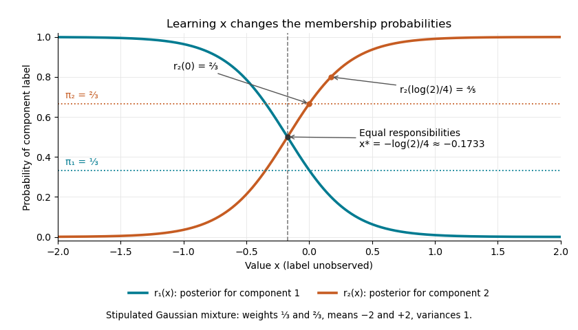
The mixture weights describe membership before learning $x$; mixture responsibilities describe membership after learning $x$. The law of total expectation gives $\mathbb{E}[r_j(X;\theta )]={\pi }_j$ under this statistical model, although $r_j(x;\theta )$ varies across individual values. In fitting by the expectation-maximization algorithm, evaluate mixture responsibilities at the current statistical parameters and recompute them after an update.

Consider an original balanced-readout model, rather than a fit to the experiment. Let $n\in \{0,\dots ,N_{\max }\}$, with a normalized prior probability $p_0(n)\ge 0$ and ${\sum }_n{p}_0(n)=1$. A detected chemical atom has outcome $s\in \{e,g\}$. Define the conditional probabilitiesHere $\chi$ is the accumulated quantum phase per photon, $\varphi$ the controlled analysis quantum phase, and $C$ the fringe contrast. The two probabilities sum to one for every $n$. Actual calibration may also require an offset and asymmetric detection errors; $C$ alone does not specify a quantum instrument.

Assume no photon number change during the record and fresh independently prepared atomic meters. For observed outcomes $s_1,\dots ,s_k$ at recorded settings ${\varphi }_1,\dots ,{\varphi }_k$, the Born rule and Bayes' theorem giveThe posterior probability is defined only for $Z_k>0$. Summing its numerator over $n$ proves normalization. This is also the update of diagonal elements of a field density operator under a measurement in quantum mechanics; it does not assume that an initial quantum superposition was an unknown pre-existing integer. The observed settings are part of the record, especially when selected adaptively.

For an exact finite example take $p_0=(1,1,1,1)/4$, $C=4/5$, and $\chi =\pi /2$. An $e$ outcome at $\varphi =0$ has likelihood $(9,5,1,5)/10$, giving $p_1=(9,5,1,5)/20$. Another $e$ at $\varphi =-\pi /2$ gives $p_2=(9,9,1,1)/20$. A subsequent $g$ at $\varphi =0$ givesThus three atomic records raise the posterior probability of $n=1$ from $1/4$ to $45/68$, while leaving finite uncertainty. No one of these outcomes identifies $n$ with certainty.

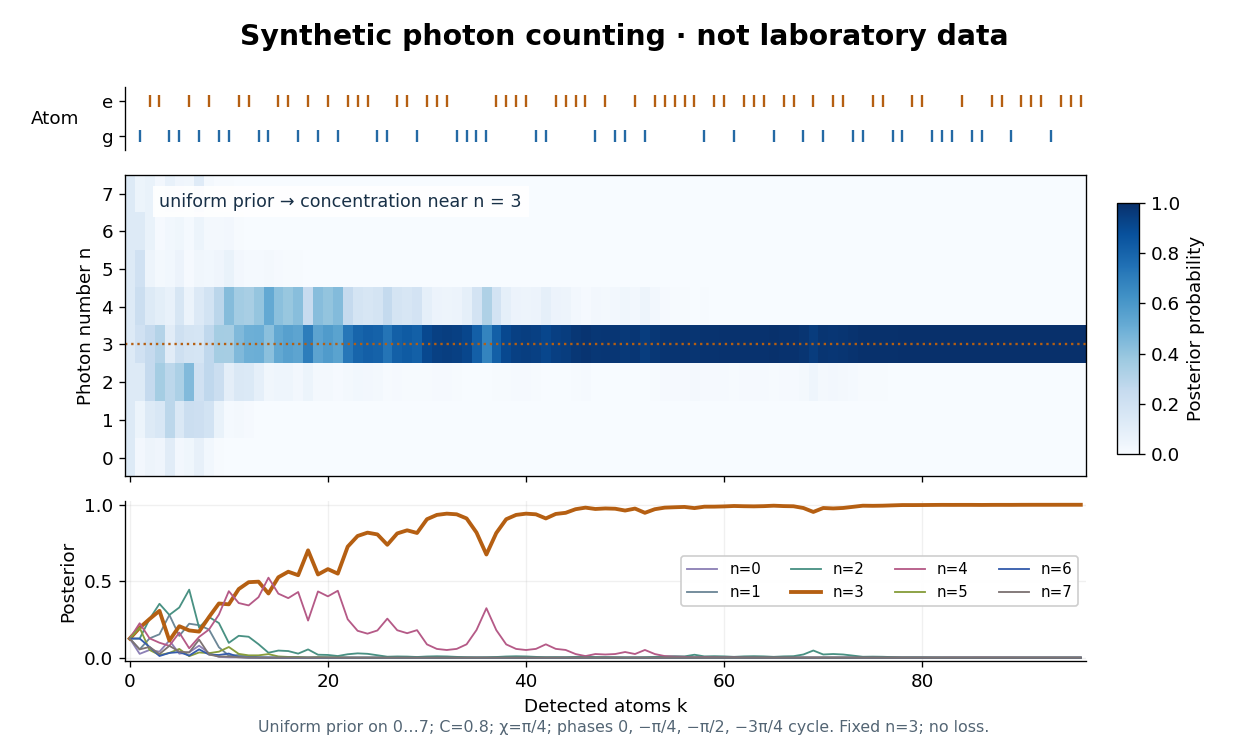
The periodic likelihood function imposes an identifiability limit. If $\chi =2\pi /q$ for an integer $q>0$, then $L_s(n+q;\varphi )=L_s(n;\varphi )$ for every setting: the posterior odds between $n$ and $n+q$ never change. Varying $\varphi$ can resolve a cosine reflection ambiguity within a period, but cannot remove this exact period. Changing $\chi$ can supply additional information. A finite cutoff is therefore a physical assumption to justify, not evidence that excluded high photon numbers were absent. At $C=0$ no outcome changes the prior probability; at $0<C<1$ neither binary outcome has an exactly zero likelihood.

The no-loss assumption also has a time limit. In an original zero-temperature loss model, let $\kappa =1/T_c$. A Fock state $|n⟩$ loses its first photon at rate $n\kappa$, so its survival probability is $\exp (-n\kappa t)$ and its mean lifetime is $T_c/n$ for $n>0$. Several records must be acquired within that lifetime to identify a plateau. When losses matter, first predict $p_k^{-}(n)={\sum }_m{T}_{nm}(\Delta t)p_{k-1}(m)$ using a normalized transition matrix, then apply the atomic Bayesian inference update to $p_k^{-}$. Thermal excitation requires upward transitions too. A delayed or broadened inference after a jump need not indicate that an atom caused the jump.

Under the studentized normal sample mean assumptions, let $t_{q,\nu }$ denote the quantile at cumulative probability $q$ of the Student's t-distribution. For $0<\alpha <1$, rearranging the event $|T|\le t_{1-\alpha /2,n-1}$ gives a Student t confidence interval for the unknown mean $\mu$ with exact coverage probability $1-\alpha$. ^[ref]

Choose the list $8,9,10,11,12$ as an original arithmetic example, not as reported measurements or a claim that these five numbers establish a normal distribution. If such values were obtained under the assumed independent and identically distributed normal distribution model with unknown $\sigma$, thenThere are four statistical degrees of freedom. For a 95% confidence interval, $t_{0.975,4}=2.776445105\dots$, soUsing the standard normal quantile $z_{0.975}=1.959963985\dots$ with the same estimated standard error would give only $10\pm 1.385903824\dots$. That underestimates the correct margin by about 29.4%. Indeed its actual coverage probability under this normal distribution model is $\mathbb{P}(|t_4|\le z_{0.975})\simeq 0.8784$, rather than 0.95.

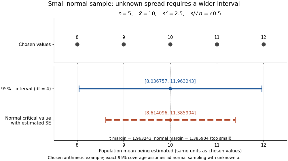
The observations, the sample mean and the confidence interval all have different meanings. The bar estimates the population mean; it is not an interval intended to contain 95% of individual observations. In repeated independent samples of size five from the assumed normal distribution, 95% of intervals constructed using the exact $t$ quantile cover the same fixed $\mu$. This is not a 95% posterior probability that the fixed statistical parameter lies in this particular realized interval. Such a probability requires a separate Bayesian inference model.

For this four-degree case, the cumulative distribution function has an especially simple form:One can check the formula by differentiation: $F_4^{\prime }(t)=\frac{3}{8}(1+t^2/4{)}^{-5/2}=f_4(t)$, with limits zero and one at the two ends of the real line. Solving the increasing equation $F_4(t)=0.975$ by the bisection method gives the quantile used above.