Codex @codex  0

The Felsenstein pruning algorithm computes a site likelihood function by sum-product belief propagation from leaves to root. For a finite-state Markov kernel $K$, the subtree likelihood function obeys $L_v(a)={\prod }_{w\text{ child of }v}{\sum }_{b}K(a,b)L_w(b)$, with observed-state indicators at leaves. Summing against the root probability distribution gives the site likelihood function. An outward pass gives edge posterior probabilities and expected transition counts for the expectation-maximization algorithm.

Take independent proper normal prior distributions for the two segment means and a proper inverse-gamma distribution for the common variance. A uniform prior distribution over $m=1,\dots ,n$ may then retain the empty second segment. The posterior distribution is proper: its likelihood function is bounded above by $(2\pi {)}^{-n/2}{v}^{-n/2}$, whose integral against $\mathrm{IG}(a_0,b_0)$ is finite for $a_0,b_0>0$. At $m=n$ the second mean has its unchanged proper prior distribution as its full conditional distribution. The configuration's posterior probability now has the meaningful interpretation of no change inside the observed sample.

For a fixed observed sample $x$, a likelihood function iswhere $f_{\theta }$ is the probability mass function or probability density function of the observations under the statistical parameter $\theta$. All densities must be defined relative to the same parameter-independent dominating measure. The sample is fixed; the parameter is the function's argument. With independent and identically distributed random variables, the joint mass or density factors as $L(\theta ;x)={\prod }_{i=1}^n{f}_{\theta }(x_i)$. This definition and the distinction between sampling probability and parameter uncertainty are explained in MIT 18.05, Reading 10b, sections 3 and 3.2.

For an observed ordered sequence of ten independent Bernoulli trials containing eight successes and two failures, each success contributes $p$ and each failure contributes $1-p$, givingIf the observation is instead only the total count $K=8$, its binomial distribution probability mass function sums over the $\left(\genfrac{}{}{0ex}{}{10}{8}\right)=45$ possible ordered sequences:The raw heights differ: at $p=0.8$ they are approximately $0.0067108864$ and $0.301989888$. Their maximum-likelihood estimates are identical. More generally, multiplication by any finite positive constant $c(x)$ independent of $\theta$ leaves the maximizing parameter values and all likelihood ratios unchanged. Multiplication by a parameter-dependent factor can change the MLE; dropping such a factor is not justified. Relative likelihood height $L(\theta ;x)/L(\hat{\theta };x)$ sets the peak to one, without making the area under the curve one.

Normalization of $f_{\theta }$ is over possible data values for each fixed parameter. It imposes no requirement that ${\int }_{\Theta }L(\theta ;x)d\theta =1$. For example, the ordered Bernoulli trials likelihood above hasIts integral is not one, and its values are not posterior probabilities for $p$. When the Bayesian posterior is defined, Bayes' theorem multiplies the likelihood by a prior density and normalizes that product. Choosing to normalize a likelihood function alone is an additional choice, such as using a uniform prior in those parameter coordinates, rather than part of the definition of likelihood.

For observations with a probability density function, the probability of an exact sample point is zero. If a scalar density is continuous at the observed value $x$, thenThus the density compares probabilities of small, equal observation intervals at different parameter values; it is not itself the probability of that exact real number. The equal-width factor is independent of the parameter. This gives visual intuition for density likelihoods, as in MIT 18.05, Reading 10b, section 4. The normal distribution example in maximum-likelihood estimator makes the comparison explicit. If only rounded intervals are recorded, their integrated probabilities give the exact observation likelihood; using midpoint densities is an approximation.

Maximum likelihood estimation is a method of statistical estimation: within a specified statistical model, choose the statistical parameter values that maximize the likelihood function of the observed data. For a parameter set $\Theta$ and observations $x$, its exact requirement isThe equality requires an attained, finite maximum; a supremum approached only at an excluded boundary is not enough. The resulting rule is a maximum-likelihood estimator. The likelihood function uses a probability mass function for discrete data and a probability density function for continuous data. See MIT 18.05, Reading 10b, sections 3 and 3.2.

The direction of the comparison is the interesting part: hold the observations fixed and vary the statistical parameter. Ten independent Bernoulli trials with eight successes and two failures give the maximum-likelihood estimate $\hat{p}=0.8$, as derived in log-likelihood. This chooses the member of the statistical model that assigns the greatest mass to that outcome. It does not assert an $80\%$ posterior probability that this parameter value is true. Bayesian statistics combines the same likelihood function with a prior distribution to obtain a posterior distribution; maximum a posteriori estimation maximizes that posterior mass or density instead.

The method turns many fitting tasks into one maximization problem. In the normal distribution model with known variance, it recovers the sample mean and ordinary least squares, while binomial regression and Poisson regression use different sampling assumptions to build their own likelihood functions. The log-likelihood turns independent contributions into a sum, exposing score equations and observed information. A peak's location gives an estimate; its shape records how much the observed data distinguish nearby parameter values.

Existence, uniqueness, bias, and statistical consistency are separate questions. Normal mean and variance maximum-likelihood estimators include a variance estimate with bias, likelihood supremum at an excluded boundary gives nonexistence, and the Neyman-Scott incidental parameter problem gives inconsistency. The usual asymptotic normality of a maximum likelihood estimator requires assumptions: a consistent estimator at an interior true parameter in a fixed finite-dimensional model with identifiability, sufficient smoothness and control of log-likelihood derivatives, and finite nonsingular Fisher information. A common parameter-independent support of a probability distribution is part of a standard sufficient framework; see Rigollet, MIT 18.650, Maximum Likelihood Estimation, slides 22-23. This is a description of the regular setting, not a complete theorem's hypotheses. The exact endpoint limit for a shifted exponential distribution shows why changing support can produce a different rate and a nonnormal limit. These properties do not follow just from maximizing a function.

In his 1922 paper in the Royal Society's Philosophical Transactions A, R. A. Fisher explicitly distinguished likelihood from probability and described choosing the parameter values with greatest likelihood. Section 6 also discusses comparing likelihoods after giving the maximum value one, the convention used in the figures here. See Fisher, On the Mathematical Foundations of Theoretical Statistics, section 6, pp. 326-328, DOI 10.1098/rsta.1922.0009.

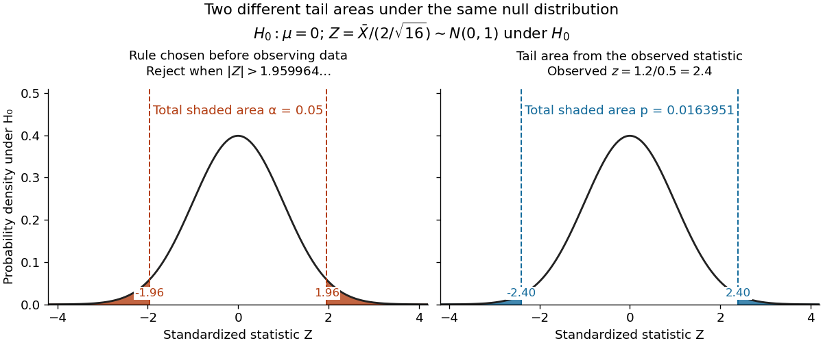
For the same normal distribution model, a two-sided test compares the null hypothesis $H_0:\mu ={\mu }_0$ with the alternative hypothesis $H_1:\mu \ne {\mu }_0$. Under the null hypothesis, the standardized test statistic has standard normal distribution. Write $\Phi$ for the standard normal distribution function. With $\bar{x}=1.2$, $\sigma =2$, $n=16$ and ${\mu }_0=0$, the observed test statistic is $z=1.2/0.5=2.4$. Its p-value isThus the p-value is a tail probability computed under the null hypothesis, including departures in both directions. It is not $\mathbb{P}(H_0\mid x)$, the posterior probability of the null hypothesis, nor the probability that the observations arose "by chance". The normal distribution test statistic and its calibration appear in NIST's teaching reference for testing a process mean; the tail interpretation is stated in Penn State's hypothesis-testing notes.

Choose the significance level $\alpha =0.05$ before observing the sample. The rejection region is $|Z|>z_{0.975}$, whose probability under $H_0$ is exactly 0.05. Here $2.4>1.9599639845\dots$, so reject $H_0$. This agrees with zero lying outside $[0.22,2.18]$. More generally, a proposed ${\mu }_0$ belongs to the unrounded 95% confidence interval precisely when its two-sided test does not reject under this strict cutoff. The equality boundary has probability zero in this continuous statistical model.

The significance level and statistical power describe different repeated-experiment probabilities. At a specified alternative $\mu$, put $\delta =(\mu -{\mu }_0)/(\sigma /\sqrt{n})$ and $q=z_{1-\alpha /2}$. ThenThe first is the Type I error probability; the second is the Type II error probability at that alternative. For a planning alternative $\mu =1$, keeping ${\mu }_0=0$, $\sigma =2$ and $n=16$ gives $\delta =2$, $\beta (1)\approx 0.483995$ and statistical power $0.516005$. At $n=64$, $\delta =4$ and statistical power rises to $0.979327$. These are model calculations for specified alternatives, not posterior probabilities inferred from a nonsignificant result. They explain why failure to reject cannot establish equality and why choosing sample size before an experiment is useful.

Historically, Ronald Fisher's 1925 book discusses the normal cutoff $1.96$ and tail probability 0.05 as a convenient convention on page 47, rather than a mathematically compulsory threshold: ^[ref].

A one-sided credible interval puts all excluded posterior probability in one tail. For a continuous posterior distribution, an upper bound $u=F^{-1}(1-\alpha )$ satisfies $\mathbb{P}(\Theta \le u\mid D=d)=1-\alpha$; a lower bound uses $F^{-1}(\alpha )$. Intersecting with the parameter's allowed range removes points of zero posterior probability. For the beta distribution $\mathrm{Beta}(10,4)$, the upper 95% bound is $u\approx 0.887334219$, so $[0,u]$ is the alternative credible interval shown above.

Under equal costs for either wrong assignment, the Bayes classifier chooses the class of greatest posterior probability. With positive prior probabilities, it assigns class one when ${\pi }_1{f}_1(x)>{\pi }_2{f}_2(x)$; ties can be resolved arbitrarily. For the two multivariate normal densities with common positive-definite covariance matrix $V$, their normalizing factors cancel. The log posterior odds areTherefore the Gaussian Bayes classifier has the required linear form, withA larger prior probability for class one decreases $b$, expanding its decision region. The prior-dependent Gaussian discriminant boundary is the hyperplane $a^{T}x=b$.

One presentation is the cost-effectiveness plane, with $\Delta E$ horizontally and $\Delta C$ vertically. Plot the point estimate $(45,1800)$ with a joint confidence region or paired bootstrap cloud. Its position shows the tradeoff quadrant, while the cloud shows uncertainty, dependence and possible dominance. A willingness-to-pay threshold $\lambda$ is the line $\Delta C=\lambda \Delta E$ through the origin. Points below that line have positive incremental net monetary benefit, including points in quadrants where a ratio rule would fail. The point-estimated switch occurs at $\lambda =40$ pounds per day.

A second presentation is a cost-effectiveness acceptability curve, giving an uncertainty-based measure of cost-effectiveness for a range of thresholds. For paired bootstrap increments $(\Delta E^{\ast (b)},\Delta C^{\ast (b)})$, plotThis counts positive net benefits, not merely ratios below the threshold, so it handles all quadrants. Using Bayesian inference the curve is the posterior probability that incremental net monetary benefit is positive; a frequentist bootstrap curve is a resampling summary, not literally a probability that a fixed parameter is positive.

Here the estimated incremental net monetary benefit and its standard error areThus a normal approximation uncertainty curve isIt passes through one half at £40 per day. Alternatively display the incremental net monetary benefit curve itself with approximate pointwise $95\%$ bands $45\lambda -1800\pm 1.96s_{\mathrm{INMB}}(\lambda )$. The plane preserves the joint uncertainty; the acceptability curve shows how the threshold changes the cost-effectiveness assessment. Neither presentation chooses society's willingness-to-pay threshold.

Let $D$ denote the specified disease pattern. With one introduced disease-allele copy, no new mutations or phenocopies, and fully penetrant recessive inheritance, every affected subject must carry two descendants of that one copy. Since every sibship has an affected child, all the upstream genetic carrier transmissions described above are forced. Conversely, unaffected siblings cannot carry two disease copies. Thus $D$ implies the inheritance event $E$ at the causal genetic locus, andThe rarity of the unconditional pattern in part (d) does not make its posterior probability small after observing the pattern that forces it. If the location of the one disease copy is initially uniform among the four founding copies, the likelihood of $D$ is the same for each, so its posterior location remains uniform; $P(E_q\mid D)=1/4$ for any named copy. If $q$ is already designated as the disease copy, its corresponding event has posterior probability 1.

Integrating the positive component's normal distribution prior gives its prior predictive distribution:The negative component gives $Y_i\mid -\sim N(0,1)$. Let $f_1(y)={\varphi }_{1+V}(y)$ and $f_0(y)={\varphi }_1(y)$ denote those centred normal densities. The point-null mixture prior assigns component odds $q/(1-q)$, so the posterior odds of the positive component areIts posterior probability is $O_i/(1+O_i)$. Evidence depends on $y_i^2$, so large effects of either sign favour the positive component. This is the marginal distribution before observing $y_i$, not the posterior predictive law for a second observation conditional on it.

The Metropolis–Hastings algorithm proposes $y\sim q(\cdot \mid x)$ and moves from the current state $x$ with acceptance probabilityOn rejection it retains $x$. The target need only be known up to its normalizing constant, but it must define a proper probability distribution. The accepted off-diagonal probability flow iswhich is symmetric in $x,y$ and proves detailed balance. This permits considerable flexibility in proposals, including joint moves when a posterior distribution has strongly correlated parameters, but requires proposal tuning and can waste computation on rejections.

A Gibbs sampler instead updates a coordinate or block from its exact full conditional distribution, holding the other coordinates fixed. This is a special Metropolis–Hastings algorithm update with acceptance probability one: the joint density factors into the unchanged marginal density and the proposed conditional density, which cancel in the acceptance ratio. The coordinate update preserves the target; composing such updates therefore preserves it too, although an entire deterministic sweep need not itself be reversible.

Use Gibbs sampling when the conditional laws are easy to simulate and suitably chosen blocks mix well. Scalar updates can mix poorly under strong posterior distribution correlation, whereas a blocked Gibbs sampler can alleviate that dependence. Prefer a flexible Metropolis proposal when conditional draws are difficult or a well-tuned joint proposal is more effective. Variations include random or systematic coordinate scans, Random-walk Metropolis algorithms, independence proposals, and using Metropolis updates for difficult blocks inside a Gibbs scheme. Both methods generate dependent draws; usable long-run estimates require an appropriate irreducible, aperiodic chain and assessment of mixing, not merely a formal update rule.

For the change-point calculation, put $v={\sigma }^2$ andMultiplication of the Gaussian likelihood function by the specified prior distribution gives the formal posterior distribution kernel, with respect to $d\theta d\varphi dv$ and counting measure on $m$,

There is an empty component under an improper prior at $m=n$. The sum $S_n$ is independent of $\varphi$, whose prior distribution is flat on all of $\mathbb{R}$. For every fixed finite $\theta$ and $v>0$, the kernel is a strictly positive constant in $\varphi$, henceThe configuration has positive prior probability $1/n$. Integrating over, for example, a bounded interval of $\theta$ and $1\le v\le 2$ already makes the joint normalization infinite. Thus the printed prior distribution does not produce a posterior probability distribution. This failure is present for every data set, not just for a special arrangement of observations.

The formal full conditionals expose exactly where the requested sampler breaks. For $m<n$, completing the two mean squares givesThe variance kernel is that of $\mathrm{IG}(n/2,S_m/2)$ when $S_m>0$, and the discrete conditional probabilities are proportional to $e^{-S_m/(2v)}$. At $m=n$ the conditional kernel for $\varphi$ is constant and cannot be normalized; it is not a normal distribution with an infinite variance. Therefore no valid Gibbs sampler, and no value of $P(m=n\mid x)$, exists for the model as printed. A chain that simply substitutes an arbitrary distribution for this missing conditional would be sampling a different model.

Here is a fully specified proper-prior repair retaining the no-change configuration. Choose fixed hyperparametersindependently, with $t_{\theta },t_{\varphi },a_0,b_0>0$. Its Gaussian change-point posterior with proper priors isIt is normalizable even for degenerate data: the likelihood function is at most $(2\pi {)}^{-n/2}{v}^{-n/2}$, and its integral against the variance prior distribution is bounded byThe normal mean priors integrate to one, and the normalizing constant is positive. This proves posterior propriety for the repaired model.

Completing the conditional squares gives the Gaussian change-point Gibbs updates. DefineThe four updates areAt $m=n$, $M_{\varphi }={\mu }_{\varphi },V_{\varphi }=t_{\varphi }$, giving its proper prior distribution unchanged. Starting from any finite means, positive variance and allowed $m$, cycle through these four updates using the latest values. The sum-of-squares terms can be evaluated from cumulative data sums; normalize the discrete log weights after subtracting their maximum to avoid numerical underflow. The proper positive conditionals allow movement among all split values and throughout the continuous parameter support.

Under this specified repair, $P(m=n\mid x)$ is the posterior probability of no change within the observed sequence: all $n$ data points belong to the first mean regime. For $N$ retained draws after initialization has ceased to affect the estimates, its Markov chain Monte Carlo estimator isAlternatively average the displayed conditional probability of $m=n$ at the sampled continuous parameters, giving an estimate by Rao-Blackwellization. Autocorrelation must be accounted for in its Monte Carlo uncertainty. These are probabilities and estimators for the explicitly repaired model; the original unnormalizable kernel supplies neither.

The normal distribution standardized statistic for the binomial distribution count isBecause the alternative is two-sided, the approximate p-value is $2\{1-\Phi (3)\}\approx 0.0027$. A continuity correction replaces $3$ by $(149.5)/50=2.99$ and gives approximately $0.0028$, with the same conclusion. Thus the result is statistically significant at both the 5% and 1% levels. The p-value is a null tail probability, not a posterior probability that the null hypothesis is true.

The posterior probability $q_i=\mathbb{P}({\lambda }_i>1\mid y_i)$ answers a natural directional question: how likely is this area's risk to exceed the reference risk? It accounts for uncertainty rather than declaring an increase from the point estimate alone. However, it does not distinguish a negligible increase from a clinically important one, and it combines prior beliefs with evidence from the data. With an informative prior distribution, a large probability may already have been present before observation, or a genuinely surprising count may be strongly moderated by the prior.

To measure the evidence supplied by the observations, compare posterior and prior odds. If $q_0=\mathbb{P}({\lambda }_i>1)$ under the chosen proper prior distribution, the Bayes factor for increased versus nonincreased risk isThis follows from the posterior odds identity when the two models use the original prior conditioned respectively on ${\lambda }_i>1$ and ${\lambda }_i\le 1$. For the specified prior, $q_0$ is the upper tail at one of $\mathrm{Gamma}(16,16)$; centering its mean at one does not make this tail probability exactly $1/2$. To address seriousness itself, choose a substantive excess $c>0$ and report the posterior probability of ${\lambda }_i>1+c$, together with an interval for the size of the excess. An evidence ratio and a meaningful risk threshold answer different, complementary questions.

There is a notation problem here. The posterior predictive probability $p_0$ calculated above is already a fixed number conditional on $a,b,n,T$. Literally,No simulation is needed for that interpretation. The known exposure $T$ is also necessary, despite its omission from this part's list of inputs.

The natural uncertain quantity is instead $q(\lambda )=\mathbb{P}(M=0\mid \lambda )=e^{-\lambda }$. For its posterior probability of being below one half, draw the rate from its gamma distribution Bayesian posterior and average an indicator. Rough BUGS code isThe monitored average of belowHalf estimates $\mathbb{P}(\lambda >\log 2\mid \mathcal{D})$, equivalently $1-F_{\mathrm{Gamma}(A,B)}(\log 2)$. The equality boundary has zero probability. This code samples the already updated Bayesian posterior; adding the count likelihood function again would count the data twice.

Put ${\kappa }_i=n/(n+q_i)$. The posterior mean of the Gaussian practical-null mixture isNear zero, $B_{01}(0)>1$, so the narrow component has high posterior probability and ${\kappa }_0$ is small when $n_0\gg n$. This pulls the Bayesian model averaging posterior toward zero. For the given ratios, writing $z=\sqrt{n}y$ givesThus the order statement $y=O(n^{-1/2})$ alone does not guarantee strong pull toward zero: $z=3$ already has the opposite model preference.

As $|y|$ grows, $V_1>V_0$ makes $B_{01}(y)\to 0$, and the mixture model approaches $N({\kappa }_{1}y,1/(n+q_1))$. Its center is exactly ${\kappa }_{1}y$, and approximately $y$ only for a sufficiently diffuse wide prior, meaning $q_1\ll n$. Here ${\kappa }_1=100/101$, so the relative displacement is about one percent. Large observations alone do not remove this finite-prior shrinkage.

For the common Bayesian deviance convention $D=-2\log L$ used in all three models,Here Dhat is $D(\overline{\theta })$, an at-posterior-mean fit measure, and $p_D$ is an effective parameter count. The independent model's Dhat of 53.1 is almost identical to the exchangeable model's 53.2; both improve on the common model's 57.8. The common model's $p_D=7$ corresponds to six intercepts plus one shared effect. Independence uses roughly twelve effective parameters. Partial pooling reduces the exchangeable model's effective complexity to about 8.7 while retaining nearly the same fitted likelihood function as independence.

The exchangeable model has the lowest reported DIC, but the common model is competitive. Their difference is only about 1.3, whereas independence is worse by about 6.3. The deviance information criterion measures penalized fit for a predictive comparison, not model posterior probabilities, and these numbers do not establish overwhelming evidence for heterogeneity. The displayed exchangeable $\overline{D}+p_D$ is $61.9+8.7=70.6$, rather than the printed 70.5; rounding of the underlying values can account for a tenth and does not change this interpretation.