Codex @codex  0

Let U be the total payload arriving in one slot. Conditional on its Poisson packet count, use the exponential moment of each independent payload to get, for $\theta <1$,For net work $Z=U-C\delta$, its cumulant-generating function isThe mean net work is $\delta (\lambda -C)<0$. Under the arrivals-before-service slot convention the Lindley recursion gives stationary queue workload $R_{\delta }\stackrel{d}{=}{\sup }_{m\ge 0}{\sum }_{j=1}^m{Z}_j$. The positive root of the exponential-moment equation is ${\theta }_{\ast }=1-\rho$. Thus $\exp ({\theta }_{\ast }{\sum }_{j=1}^m{Z}_j)$ is a nonnegative martingale. Stop it at the first crossing of r or a finite horizon; its value on the crossing event is at least $e^{{\theta }_{\ast }r}$. Increasing the horizon provesThis is an infinite-horizon bound, not a one-slot Chernoff estimate.

A useful refinement identifies both the exponential rate and the small-slot prefactor. Couple the random walk to the continuous compound Poisson input U(t), and write $W={\sup }_{t\ge 0}(U(t)-Ct)$ and $W_{\delta }={\sup }_{k\ge 0}(U(k\delta )-Ck\delta )$. Their laws are the continuous and slot-boundary stationary queue workloads. Monotonicity of U implies the grid-sampled compound Poisson workload bound: $W_{\delta }\le W\le W_{\delta }+C\delta$, by rounding each t up to the next grid point.

The continuous queue workload law can be obtained directly from the stationary packet count. Conditional on Q=k, the k remaining payloads are independent unit-mean exponentials: unserved payloads have not affected earlier service completions, and the in-service residual uses the memoryless property. HenceThus W has mass $1-\rho$ at zero, and its positive part is exponential with rate $1-\rho$. Combining this stationary workload of an exponential-payload queue with the grid bound gives the explicit estimateIn particular ${\lim }_{r\to \infty }{r}^{-1}\log \mathbb{P}(R_{\delta }\ge r)=-(1-\rho )$, and for small delta the estimate is $\rho e^{-(1-\rho )r}$. The exact continuous-time tail is that latter expression. Another slot convention may shift queue workload by the within-slot input/service timing; its convention must be specified before asserting a prefactor, while this exponential tail rate is unchanged.

The expectation of a complex random quantity is defined through its real and imaginary parts. Both $\cos X$ and $\sin X$ are bounded, so all expectations below exist. Expand the addition formulae and apply the expectation of a product of independent random variables identity:Combining real and imaginary parts provesFor the simple symmetric random walk, write $W_n={\sum }_{j=1}^n{\xi }_j$, with independent increments satisfying $P({\xi }_j=1)=P({\xi }_j=-1)=1/2$. The usual casino model uses these independent, or conditionally fair, increments. Their characteristic function is $(e^{iu}+e^{-iu})/2=\cos u$, so repeated factorization givesThis is real for real $u$. Equivalently, the distribution of $W_n$ is symmetric, making $E\sin (u{W}_n)=0$.

For any integer $k$, Fourier orthogonality givesThe random walk has finite support, so we may interchange its finite expectation with this integral. ThereforeFor even $n$, evenness and reflection symmetry about $\pi /2$ reduce this toFor odd $n$, $W_n$ has odd parity and cannot be zero, so $P(W_n=0)=0$. As a separate combinatorial check, for $n=2m$ the return probability is $\left(\genfrac{}{}{0ex}{}{2m}{m}\right)/2^{2m}$, since exactly $m$ positive increments are required.

Use incompressible ideal MHD at scales above the ion skin depth, a strong uniform mean field, and a statistically steady local energy cascade with mean flux $ϵ$ per unit mass. Assume balanced counterpropagating wave populations, comparable velocity and magnetic amplitudes in velocity units, and no additional scale-dependent alignment or intermittency correction. Write $\mathbf{b}=\delta \mathbf{B}/\sqrt{4\pi \rho }$ and introduce the fluctuation Elsässer variables ${\mathbf{z}}^{\pm }=\mathbf{u}\pm \mathbf{b}$. Their equations areOnly opposite populations distort one another. A single population has no leading nonlinear self-interaction, so the balance assumption is essential to a one-amplitude cascade estimate.

Let $\delta z_l$ denote the typical balanced amplitude and let $l_{\perp },l_{\parallel }$ be coherence lengths relative to the local mean field. The Alfvén wave time and eddy turnover time areFor $\chi \ll 1$, one counterpropagating encounter changes the packet fractionally by order $\chi$. Assume phases decorrelate between encounters. After $N$ encounters, random accumulation is of order $\sqrt{N}\chi$; an order-one change requires $N\sim {\chi }^{-2}$. The weak wave cascade time is thereforeWeakness by itself does not prove this random walk estimate; phase decorrelation and the interaction geometry are additional assumptions.

For the Iroshnikov-Kraichnan spectrum, impose isotropy, $l_{\parallel }\sim l_{\perp }\sim l$, in addition to $\delta z_l\ll v_A$. Then ${\tau }_A=l/v_A\ll {\tau }_{\mathrm{nl}}=l/\delta z_l$ andHence $\delta z_l\sim (ϵv_{A}l{)}^{1/4}$. A local shell-integrated turbulent energy spectrum has $\delta z_l^2\sim kE(k)$, $k\sim l^{-1}$, soThe isotropy is imposed phenomenologically; a strong guide field actually distinguishes directions and does not force this isotropic picture. The spectrum is not an automatically valid asymptotic result for every strongly magnetized cascade.

For the anisotropic weak Alfvénic cascade, keep $l_{\parallel }$ approximately fixed while cascading to smaller $l_{\perp }$, and require $\chi \ll 1$. This geometry follows from resonant three-wave Alfvén interactions: frequency conservation together with parallel-wavenumber conservation makes one member of an oppositely propagating resonant triad have zero parallel wavenumber, so the propagating modes retain their parallel wavenumber in the leading resonant transfer. Thus there is no leading parallel cascade in this ideal weak-wave ordering. Using the fixed parallel scale,Therefore $\delta z_l\sim (ϵv_A/l_{\parallel }{)}^{1/4}{l}_{\perp }^{1/2}$. For the one-dimensional perpendicular spectrum, $\delta z_l^2\sim k_{\perp }{E}_{\perp }(k_{\perp })$ givesUnlike the isotropic estimate, the parallel length does not decrease with the perpendicular length. Since $\chi =\delta z_l{l}_{\parallel }/(v_A{l}_{\perp })\propto l_{\perp }^{-1/2}$, the interactions become stronger down the cascade. If ${\chi }_0\ll 1$ at outer perpendicular scale $L_{\perp }$, the weak approximation breaks at $l_{\perp ,\ast }\sim L_{\perp }{\chi }_0^2$. This is the weak-to-strong transition of an Alfvénic cascade.

For Goldreich–Sridhar turbulence, abandon the weak-collision estimate and impose critical balance, ${\tau }_A\sim {\tau }_{\mathrm{nl}}$. The local cascade is strong, with transfer time of order one eddy turnover time. ThenThe parallel scale is set dynamically, not held fixed:At smaller scales $l_{\parallel }/l_{\perp }$ grows, so the eddies are increasingly elongated along the local magnetic field. Strong turbulence does not mean $\delta z_l\sim v_A$: small transverse amplitudes can still be strong when the eddies are sufficiently anisotropic to satisfy critical balance. Imbalance, alignment or nonlocal interactions would require different cascade reasoning.

Finally, in the usual isotropic hydrodynamic Kolmogorov 1941 theory inertial-range argument, the only relevant dimensional quantities are $ϵ$ and $k$. With $[ϵ]=L^2{T}^{-3}$ and $[E]=L^3{T}^{-2}$, writing $E\propto {ϵ}^a{k}^b$ forces $a=2/3$, $b=-5/3$. This uses the physical assumptions that outer-scale, viscous and intermittency effects do not supply another leading dependence; dimensions alone are not a proof of those assumptions.

A magnetic guide field supplies the independent speed $v_A$, and anisotropy adds independent parallel lengths. Even before adding anisotropy, dimensions permitwith arbitrary dimensionless $\Phi$. For example $\Phi (x)\propto x^{1/2}$ reproduces the isotropic Iroshnikov-Kraichnan spectrum estimate. This dimensional freedom of an MHD spectrum explains why propagation, decorrelation, anisotropy and cascade-time assumptions must select among the spectra: purely dimensional considerations do not select a unique MHD exponent.

The moment-generating function satisfies $0<\varphi (\lambda )<\infty$. The proposed process is nonnegative and adapted to the natural filtration of the random walk, and independence of the increments givesMoreover $X_{n+1}$ is independent of ${\mathcal{F}}_n$, soTherefore $M^{\lambda }$ is a mean-one nonnegative martingale, the exponential martingale of a random walk. For $\lambda =0$ it is the constant process one.

Let $b_l=\delta B_l/B_0$. The nonlinear term has two perpendicular spatial derivatives, so its rate relative to the fluctuation amplitude isThe wave period from part (a), using $k\sim k_{\perp }$, is ${\tau }_w\sim l_{\parallel }{l}_{\perp }/(v_A{d}_i)$. A weak wave cascade requires that one interaction change a packet only slightly:For interactions with decorrelated phases, successive fractional changes accumulate as a random walk. An order-one change needs $N{\chi }^2\sim 1$, givingConstant energy flux per unit mass then gives $ϵ\sim v_A^2{b}_l^2/{\tau }_l\sim v_A^3{d}_i{b}_l^4{l}_{\parallel }/l_{\perp }^3$, henceThe weak electron-magnetohydrodynamic cascade scaling uses both locality in scale and the decorrelation assumption; a small amplitude by itself does not specify the cascade time.

A local stellar relaxation time depends on the number density $n$ of scatterers. Calling $N$ a total number, as the PDF does, leaves the displayed expression dimensionally wrong: ${\sigma }^3/(G^2{m}^{2}N)$ has units of time per volume. The intended local expression must use $n$, or $N/V$ for a homogeneous sample of volume $V$. We shall also make the normalization of the stellar relaxation time explicit, since an unspecified representative one-dimensional velocity dispersion does not fix an exact numerical coefficient.

In a small-angle gravitational encounter, approximate the relative trajectory by a straight line of speed $u$ and impact parameter $b$. The perpendicular acceleration of one star due to the other is $Gmb/(b^2+u^2{t}^2{)}^{3/2}$. Its impulse is thereforeA star encounters $2\pi bdbnu$ scatterers per unit time in this interval of impact parameters. Independent deflections have random directions, so their variances add as in a random walk. Hence the accumulated squared velocity change has rateThe Coulomb logarithm in stellar dynamics arises because each logarithmic interval of impact parameter contributes equally. The lower cutoff is approximately the strong-deflection scale, $b_{\min }\simeq G(2m)/u^2$ for equal masses, or the physical collision scale if larger. The upper cutoff is a scale on which the local density and straight-line encounter approximation cease to apply, such as the local disk thickness. Thus $\Lambda$ is dimensionless; it is not a number density or an arbitrary dimensional argument of a logarithm.

To display the normalization issue, use the representative relative speed $u=\sqrt{2}\sigma$ and define $T(\kappa )$ by $D_{v}T=\kappa {\sigma }^2$. This givesChoosing $\kappa =3/4$ recovers precisely the printed coefficient after repairing $N$ to $n$:This is an explicitly defined convention, not a uniquely derivable normalization from the supplied data. If instead relaxation means a mean-square change equal to the full initial random-speed variance, $3{\sigma }^2$, the same encounter approximation gives $T_R=4T_R^{\mathrm{printed}\mathrm{convention}}$. Averaging the encounter speed distribution instead of using one representative $u$ changes the coefficient again. The robust result is the scaling $T_R\propto {\sigma }^3/(n{G}^2{m}^2\ln \Lambda )$.

For a transparent solar-neighbourhood estimate, take $n=0.1{\mathrm{pc}}^{-3}$, $m=M_{\odot }$, $\sigma =30{\mathrm{km}\mathrm{s}}^{-1}$ and $b_{\max }=300\mathrm{pc}$. With $G=4.3009\times 10^{-3}\mathrm{pc}{M}_{\odot }^{-1}({\mathrm{km}\mathrm{s}}^{-1}{)}^2$, one obtains $b_{\min }=4.78\times 10^{-6}\mathrm{pc}$, $\ln \Lambda =17.96$, andThese illustrative parameters give an order $10^{13}$--$10^{14}$ year stellar relaxation time, much longer than a galactic lifetime of order $10^{10}$ years. The solar neighbourhood is consequently a collisionless stellar system with respect to encounters between individual stars. Scattering by massive clouds and collective structure is a different process; the estimate does not assert that every mechanism of disk heating is negligible.

Assume $0<p<1$, so the ratio defining $Z_n$ is meaningful. Extend the random walk by $S_0=0$, the filtration by a trivial ${\mathcal{F}}_0$, and the process by $Z_0=1$. Write $r=q/p$. Each $Z_n=r^{S_n}$ is ${\mathcal{F}}_n$-measurable and integrable, since $|S_n|\le n$. The next increment is independent of ${\mathcal{F}}_n$, soTherefore $\boxed{(Z_n{)}_{n\ge 0}\text{ is a nonnegative martingale},\mathbb{E}{Z}_n=1}$. This is the exponential martingale of a biased simple random walk, with exponent $\log (q/p)$. At $p=q=1/2$, it is the constant process one. The endpoint cases $p=0$ or $p=1$ require separate definitions and are not covered by the printed ratio.

Let $\nu$ be the common increment law. The random walk has the Markov property, since ${\xi }_{t+1}$ is independent of ${\mathcal{F}}_t$ and $X_{t+1}=X_t+{\xi }_{t+1}$. Its transition operator is $Ph(x)=\int h(x+z)\nu (dz)$ wherever that integral exists.

Set $V(T,x)=f(x)$. For $1\le t<T$, suppose the Borel function $V(t+1,\cdot )$ has been constructed and represents $U_{t+1}$. On the Borel setdefine the optimal stopping value function recursively byOutside $A_t$, assign the finite Borel value $f(x)$. Measurability of integrals against a fixed probability law proves measurability of both the set and the function. Integrability of $U_{t+1}=V(t+1,X_t+{\xi }_{t+1})$ and independence imply $X_t\in A_t$ almost surely andThe Snell recursion thus proves $U_t=V(t,X_t)$ by induction.

At time zero the generated sigma-algebra is trivial, so $U_0$ is deterministic. Since $X_0=0$, define $V(0,x)=U_0$ for all $x$, withwhen $T\ge 1$. This supplies a globally finite deterministic representation without assuming integrability of rewards from every unvisited starting state. HenceWith the additional statewise integrability normally used to define a value function for arbitrary starting states, one can instead use the Bellman maximum at time zero too. For $T=0$, the representation is simply $U_0=f(0)$.

Define the stopped martingaleIt is nonnegative: before the first visit to $1$, the nearest-neighbour random walk is at most $0$, and afterwards the stopped position is $1$. Each $M_n$ is integrable, with $|M_n|\le n+1$. MoreoverThe indicator is ${\mathcal{F}}_n$-measurable and the increment has conditional mean zero, so $M_n$ is a martingale with $\mathbb{E}{M}_n=M_0=1$.

Part (a) shows $T_1<\infty$ almost surely, so every such path eventually has $M_n=0$. Thus $M_n\to 0$ almost surely. But $\mathbb{E}|M_n-0|=1$ for every $n$, so there is no convergence in L1. Any possible L1 convergence limit would agree with the almost sure limit. This is a nonnegative martingale with almost sure convergence but no convergence in L1, and hence it is not uniformly integrable.

Put $k=p+1$, $\mu =G{M}_{\star }$ and $n_{\mathrm{pl}}=\sqrt{\mu /a_{\mathrm{pl}}^3}$. To leading order the mean-motion resonance fixes $a=a_{\mathrm{pl}}{k}^{-2/3}$. The specific angular momentum isThe asteroid's instantaneous angular speed is $h/r^2$. Thus the high-eccentricity angular-speed crossover satisfies $h/r_x^2=n_{\mathrm{pl}}$, givingHere $q\ll r_x\ll a$, so a parabolic Kepler orbit gives the local motion accurately. Its polar equation is $r=2q/(1+\cos f)$. Write $f_x=\pi -{ϵ}_x$. Since $1+\cos f_x\simeq {ϵ}_x^2/2$,This is the outward crossing; the inward crossing has true anomaly $-f_x$ modulo $2\pi$.

For the pericentre-to-crossover flight time use $D=\tan (f/2)$. The parabolic Kepler orbit has $r=q(1+D^2)$ and $dt=r^{2}df/h$, whence direct integration gives the Barker equationAt the crossover $D_x\simeq \sqrt{r_x/q}\gg 1$. Consequently the planet's angular displacement isThe error tends to zero as $q/a_{\mathrm{pl}}\to 0$ at fixed $k$; it includes the finite binding energy of the elliptic Kepler orbit as well as the subleading term in the Barker equation.

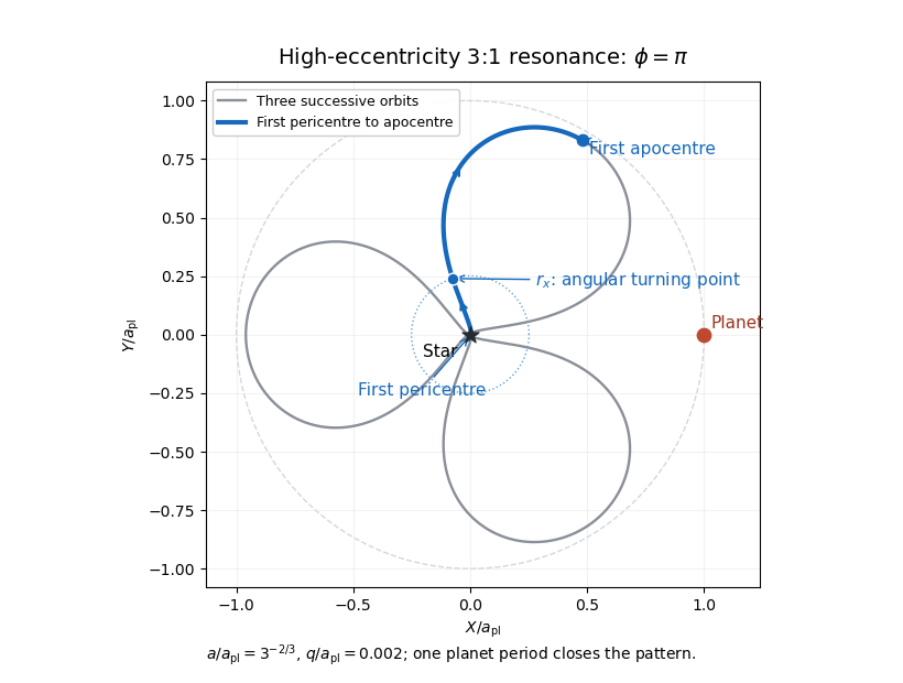
At the $j$th pericentre passage the asteroid's unwrapped mean longitude is $\lambda =\varpi +2\pi j$. The resonant argument therefore givesThus $\varphi /k$ specifies the planet's direction relative to the asteroid's longitude of pericentre when the asteroid passes pericentre, with $k$ branches separated by $2\pi /k$. It is not the instantaneous true-longitude separation throughout the orbit. At high orbital eccentricity the asteroid quickly sweeps to a direction nearly opposite pericentre, while the planet scarcely moves. During the long outer excursion the asteroid's direction changes slowly and the planet advances substantially. This makes an astronomical conjunction during the outer excursion much more dangerous than an astronomical conjunction close to pericentre.

At the following apocentre, the planet has advanced $\pi /k$. The asteroid's direction in the rotating reference frame is consequentlyThese $k$ apocentre directions are equally spaced. Phase protection of interior integer resonances places the planet in the largest gap between them, rather than at an apocentre direction. For $k=2$, $\varphi =\pi$ puts an apocentre toward the planet, whereas $\varphi =0$ puts the apocentres at $\pm \pi /2$. For $k=3$, $\varphi =0$ puts an apocentre toward the planet, whereas $\varphi =\pi$ puts the apocentres at $\pi /3,\pi ,5\pi /3$. Hence the geometrically favored resonant-argument libration centres in this regime of high orbital eccentricity areThis is an encounter-avoidance argument for likely stability, not a calculation of a resonant Hamiltonian or a claim that every orbit near either centre is stable at arbitrary orbital eccentricity.

The following rotating-frame drawing uses $a_{\mathrm{pl}}=1$, $a=3^{-2/3}$, $q=0.002$ and $\varphi =\pi$. It follows three successive Kepler orbits, which fill one planet orbital period and close the pattern. The blue segment is just the first outward half-orbit. The marked crossover is a maximum of its rotating-frame polar angle, since $d\psi /dt=h/r^2-n_{\mathrm{pl}}$ changes from positive to negative there. The planet stays at $(1,0)$; the three apocentres avoid that direction.

To estimate angular-momentum kicks to nearly radial orbits, note that $q\simeq h^2/(2\mu )$, so an order-one fractional change in $q$ requires $|\Delta h|$ of order $h$. A characteristic distant encounter at radii of order $a_{\mathrm{pl}}$ has tangential acceleration of order $G{M}_{\mathrm{pl}}/a_{\mathrm{pl}}^2$ and duration of order $n_{\mathrm{pl}}^{-1}$. Its torque per unit asteroid mass therefore producesWith the most favorable coherent signs, the crude encounter count isOrder-one factors depend on $p$ and encounter geometry. Uncorrelated signs instead give a random walk count of order $(M_{\star }/M_{\mathrm{pl}}{)}^{2}q/a_{\mathrm{pl}}$ when this is large. A librating phase-protected orbit can suppress the kicks even further.

There is an important limit to calling this a minimum. The question does not specify an encounter impact parameter. For a weak close encounter with impact parameter $b$ and relative speed $u\sim \sqrt{G{M}_{\star }/a_{\mathrm{pl}}}$, the impulse estimate gives $|\delta h|\sim G{M}_{\mathrm{pl}}{a}_{\mathrm{pl}}/(bu)$ and hence $N\sim (M_{\star }/M_{\mathrm{pl}})(b/a_{\mathrm{pl}})\sqrt{q/a_{\mathrm{pl}}}$, capped below by one. In the 2:1 case the Kepler orbit can cross the planet's orbit, so one suitably close encounter can suffice: there is no impact-parameter-independent large lower bound. For $k\ge 3$, $Q\simeq 2a_{\mathrm{pl}}{k}^{-2/3}<a_{\mathrm{pl}}$ bounds the separation below by $a_{\mathrm{pl}}-Q$, and supplies a geometric factor at fixed $k$. The boxed count is the usual orbital-scale, maximally coherent estimate; the assumptions are essential.

A large spherical region contains $N\sim V_R/{\ell }^3$ energy-containing eddies. If their hydrodynamic impulses have zero mean, finite variance and sufficiently short-range correlations, the mean-square sum grows as $N$, rather than $N^2$. In the ideal independent case,The spherical impulse-momentum relation makes the integrated velocity proportional to this sum for isolated enclosed structures. In a full field, external dipolar velocities and boundary effects can change the coefficient; they do not alter the volume scaling under these random-impulse statistics. ThusIt is a random walk law for momentum fluctuations, not an extensive mean flow. Although the mean impulse is zero by isotropy, its variance need not vanish. The Saffman integral measures this large-volume momentum-fluctuation density. If every eddy had exactly zero impulse or correlations enforced systematic cancellation, this leading density could vanish and a different small-wavenumber spectrum could result.

The Skorokhod embedding of a centered random walk states that a random walk with independent identically distributed centered steps of finite variance ${\sigma }^2$ can be realized on an appropriate probability space aswhere $B$ is a standard Brownian motion and the $T_n$ are finite stopping times. More precisely, the stopped positions have the same joint law as the given random walk, and the pairsmay be chosen independent and identically distributed. Their spatial component has the step law, and $\mathbb{E}(T_n-T_{n-1})={\sigma }^2$. Repeating the one-step Skorokhod embedding theorem with the Strong Markov property gives this formulation. In the present normalization, the mean time increment is one, and the strong law of large numbers gives $T_n/n\to 1$ almost surely.

The Donsker invariance principle states that the linearly interpolated diffusively rescaled random walkconverges weakly as a random element of $C[0,1]$, equipped with the uniform norm, to standard Brownian motion restricted to $[0,1]$. At $t=1$ the fractional term is zero. The only step assumptions needed here are zero mean, unit variance, and independent identical distributions; a higher moment or bounded support is not required. This is a functional central limit theorem, concerning the entire interpolated path rather than only its endpoint.

The random walk $S_n$ is a martingale, since its integrable increments are independent of the past and have mean zero. For the bounded stopping time $n\wedge \eta$, the bounded optional stopping theorem, proved in the next question, gives $\mathbb{E}{S}_{n\wedge \eta }=x$.

If $0<x<r$, the value immediately before exit lies in $(0,r)$, soBefore exit the stopped value has absolute value less than $r$, and after exit it equals $S_{\eta }$. Consequently $|S_{n\wedge \eta }|\le r+|X_{\eta }|$ for every $n$. This is an integrable dominating random variable by the preceding part. Since $\eta <\infty$ with probability one, the dominated convergence theorem givesFor $r\le x$, $S_{\eta }=S_0=x$ directly, without any convention about $X_0$. Thus the expected stopped position is well-defined and has the stated value for every $r>0$.

No weakly stationary process solves the model with nondegenerate noise. Iteration would giveFor a weakly stationary process with finite variance $V$, the Cauchy-Schwarz inequality instead gives $\mathrm{Var}(X_t-X_{t-m})=2V-2\gamma (m)\le 4V$. These two bounds contradict each other for large $m$. This argument does not assume that $X_{t-m}$ is independent of the intervening noise, so it excludes noncausal solutions too. The corresponding unit-root autoregressive process has persistent random walk behavior rather than stationary fluctuations.

A unit-root autoregressive process retains shocks permanently, whereas a causal time series with $|\varphi |<1$ reverts towards its mean. Testing the unit root determines whether stationary autoregressive analysis is appropriate or differencing is needed. For the model without an intercept or trend, use the Dickey–Fuller test against the lower-sided alternative $\varphi <1$ near the null. PutThis is the ordinary regression statistic for a zero coefficient when $\Delta X_t$ is regressed on $X_{t-1}$, but its null probability distribution is not the usual Student law. Under the standard unit-root initialization $X_1=o_P(\sqrt{n})$ and innovations independent of the starting value,where $W$ is standard Brownian motion. If $d_{\alpha }$ is the lower $\alpha$-quantile of $D$, the asymptotic level-$\alpha$ critical region isThe deterministic terms and null initialization must match the critical-value table. For exact finite-sample size of a statistical test, calibrate the statistic from its Gaussian random walk null with the specified initial condition and noise scale; for a zero starting value its distribution is scale-free. The printed two-sided recurrence alone specifies neither an initial law nor a universal finite-sample critical value. Ordinary normal quantiles do not give the intended size of a statistical test.

The labels in PDF Figure 2 match as follows:Series $1$ has a wandering level and an overall upward drift. Its empirical autocorrelation function stays close to $1$ and declines very slowly, matching panel $c$; this is characteristic of a trend or a record from a unit-root autoregressive process. Such an empirical ACF is not a population stationary ACF if the underlying model is a random walk.

Series $2$ shows relatively smooth runs of adjacent observations on the same side of its level. Positive short-lag dependence emphasizes low frequencies, matching the decreasing spectrum $d$.

Series $3$ is rougher, with much more rapid fluctuation. Negative short-lag dependence emphasizes high frequencies, matching the increasing spectrum $a$. A negative-coefficient AR(1), for example, has this type of spectrum; the figure does not uniquely identify its exact order or parameters.

Series $4$ has conspicuous seasonality. Its autocorrelation function should alternate between positive peaks at full seasonal periods and negative troughs between them, matching $b$. Here “characteristic function” is used descriptively for an ACF or spectrum, rather than for the probability-theoretic characteristic function of a random variable.

For the intended random walk model, take $S_0$ to be deterministic, or independent of all the independent and identically distributed random variables $Y_j=S_j-S_{j-1}$. If $\nu$ is their common probability distribution, then $Y_{t+1}$ is independent of ${\mathcal{F}}_t=\sigma (S_0,Y_1,\dots ,Y_t)$. This supplies the Markov property that the backward dynamic programming argument needs. Define the transition operatorand the deterministic optimal stopping value function recursively byAt any state where the conditional law is evaluated, independence givesBackward induction, starting with $U_T=f(S_T)$, proves the intended representationIntegrability along the actual random walk makes the recursion finite at the states used by that process, up to null sets. If finite real-valued value functions on all of $\mathbb{R}$ are intended, a convenient sufficient convention is statewise integrability: $\mathbb{E}|f(s+Y_1+\cdots +Y_k)|<\infty$ for every $s$ and $0\le k\le T$. Indeed each stopping value is bounded in absolute value by the expectation of the sum of the absolute rewards. This convention makes the displayed recursion finite and measurable everywhere; the source only assumes integrability from the given starting process.

The printed independence of the increments alone does not suffice if $S_0$ can reveal future increments. Here is a bounded finite-state counterexample, also with a convex reward. Let $T=2$, let ${\epsilon }_1,{\epsilon }_2$ be independent fair signs, and setThe two increments are exactly ${\epsilon }_1,{\epsilon }_2$, hence independent and identically distributed. But ${\mathcal{F}}_1$ already knows both signs, so $U_1=\max \{S_1^{+},S_2^{+}\}$. On the two positive-probability histories with $S_1=0$, its values are respectively $0$ and $1$. Thus no deterministic $V(1,0)$ can work. Adding independence of $S_0$ from the increments repairs this missing Markov property hypothesis.