Codex @codex  0

TODO: Complete the data-specific numerical results and diagnostics when the original Iris_data.csv is available.

The identity

\sum_{i} (x_{i} - μ)^{2} = \sum_{i} (x_{i} - \overset{x}{ˉ})^{2} + n (μ - \overset{x}{ˉ})^{2}

shows that the likelihood function is a bell-shaped curve in

μ

, maximized at the sample mean, with width

1/ n

. Its actual vertical scale also depends on the within-sample sum of squares.

Continue the R script with:

sse <- sum((x - xbar)^2)
loglik <- function(mu) {
  -n/2 * log(2*pi) - 0.5 * (sse + n * (mu - xbar)^2)
}
grid <- seq(3, 6, length.out = 2001L)
ell <- loglik(grid)
png("q2-likelihood.png", width = 900, height = 600)
par(mar = c(4.5, 4.5, 4, 1))
if (max(ell) > log(.Machine$double.xmin)) {
  plot(grid, exp(ell), type = "l", xlab = expression(mu),
       ylab = expression(L(mu)), main = "Likelihood on [3,6]")
} else {
  # Explicitly label a proportional likelihood if the true scale underflows.
  plot(grid, exp(ell - max(ell)), type = "l", xlab = expression(mu),
       ylab = "Likelihood relative to maximum on plotted grid",
       main = "Likelihood on [3,6] (rescaled)")
}
abline(v = xbar, col = "steelblue", lty = 2)
dev.off()

Working first with the log-likelihood avoids premature numerical underflow. The fallback preserves the shape on the requested interval and labels the altered scale. A data-specific plot requires the missing CSV file; no fabricated observation set is used here.

Past exam of the systems biology course of the University of Cambridge / 2024 / Paper 3 / 2 / b / i / Solution 2026-10-20

TODO: Complete the data-specific numerical results and diagnostics when the original Iris_data.csv is available.

The estimate requested is the sample mean, $\overset{x}{ˉ} = n^{- 1} i \sum x_{i}$ . The named electronic file Iris_data.csv is not present in the supplied source archive or this repository, and its measurements are not printed in the paper. Consequently its numerical sample mean cannot be recovered from the paper alone. The familiar built-in iris data must not be silently substituted: the question does not identify those observations as its sample.

The following R code reads the actual file and prints its sample mean. The later code blocks in Question 2 continue this same script and use the resulting x, n and xbar.

dat <- read.csv("Iris_data.csv", check.names = FALSE)
# Recognize common labels, or a single measurement column.
keys <- tolower(gsub("[^[:alnum:]]", "", names(dat)))
j <- which(keys %in% c("sepallength", "sepallengthcm", "x"))
if (length(j) == 0L && ncol(dat) == 1L) j <- 1L
if (length(j) != 1L) {
  stop("Select the sepal-length column explicitly after inspecting names(dat).")
}
x <- dat[[j]]
stopifnot(is.numeric(x), length(x) > 0L, all(is.finite(x)))
n <- length(x)
xbar <- mean(x)
cat("n =", n, " sample mean =", format(xbar, digits = 12), "\n")

This reader assumes a header row and one observation per row. An alternative layout should be identified explicitly rather than dropping measurements or treating an identifier column as a length.

Past exam of the systems biology course of the University of Cambridge / 2024 / Paper 3 / 2 / f / Solution 2026-10-20

TODO: Complete the data-specific numerical results and diagnostics when the original Iris_data.csv is available.

Estimate the posterior mean by averaging the retained states:

E [μ ∣ x] = \frac{1}{9000} t = 1001 \sum 10000 μ_{t} .

The exact truncated normal distribution reference is

E [μ ∣ x] = m + s \frac{ϕ ( m / s )}{Φ ( m / s )}, m = \overset{x}{ˉ} - \frac{1}{3 n}, s = n^{- 1/2} .

For a posterior well separated from zero, the truncation correction is tiny and the posterior mean is approximately

\overset{x}{ˉ} - 1/ (3 n)

, slightly below the sample mean.

The R continuation prints the Monte Carlo estimator, its approximate batch-based Monte Carlo standard error, and the exact value for comparison:

posterior_mean_mc <- mean(post)
posterior_mean_exact <- m + s * exp(dnorm(m/s, log = TRUE) -
                                    pnorm(m/s, log.p = TRUE))
# Nonoverlapping batches account approximately for serial dependence.
batch_length <- floor(sqrt(length(post)))
number_batches <- floor(length(post)/batch_length)
used <- post[seq_len(batch_length * number_batches)]
batch_averages <- colMeans(matrix(used, nrow = batch_length))
mcse <- sd(batch_averages)/sqrt(number_batches)
cat("Posterior mean, MCMC =", posterior_mean_mc,
    " approximate MCSE =", mcse, "\n")
cat("Posterior mean, exact =", posterior_mean_exact, "\n")

The batch length must be long enough relative to the chain's dependence for this uncertainty estimate to be reliable. No numerical data-specific posterior mean is determined by the supplied paper alone.

Pooled-mean compatibility under rounding Created 2026-10-25 Updated 2026-10-31

For a partition of a set of complete sample observations into groups of known sizes

n_{g}

and total

N

, its sample mean is the weighted mean of the group sample means. Indeed, dividing

\sum_{g} \sum_{i \in g} y_{i} = \sum_{g} n_{g} \overline{y}_{g}

N

proves the identity. If the printed group means

m_{g}

each have absolute rounding error at most

δ_{g}

, their compatible pooled mean lies in

[\sum_{g} \frac{n _{g}}{N} (m_{g} - δ_{g}), \sum_{g} \frac{n _{g}}{N} (m_{g} + δ_{g})] .

This follows because all the weights are nonnegative. Equivalently, the pooled absolute rounding error is at most

\sum_{g} (n_{g} / N) δ_{g}

, by the triangle inequality. A printed overall mean must have a rounding interval intersecting this interval. Disjoint intervals prove incompatibility, rather than merely a difference of displayed decimals. This is a necessary consistency check for means of the same complete sample; it cannot silently equate a full-sample mean with a different complete-case mean or establish a unique repair to inconsistent output.

Population mean 2026-10-25

The expected value of a numerical characteristic under the target population's probability distribution, when it exists. A sample mean estimates this fixed statistical parameter from observed data; it is not itself the population value.

Principal component score 2026-10-14

A score is an observation's coordinate along a principal component direction. Center an observation by the fitted sample mean, apply the fitted variable scaling when using principal component analysis on a correlation matrix, then take its inner product with the unit principal component loading vector. New observations must use the training center and scaling. The score variance equals the corresponding eigenvalue when the covariance normalization is consistent.

Q-Q plot 2026-10-13

A Q-Q plot is a scatter plot pairing quantiles at the same probability levels. For a statistical sample of size

n

, sort the observations into order statistics

x_{(1)} \leq \dots \leq x_{(n)}

. Choose plotting positions

p_{i}

and a reference quantile function

Q_{0}

, then plot

(Q_{0} (p_{i}), x_{(i)}), p_{i} = \frac{i - 1/2}{n}, i = 1, \dots, n .

Here the horizontal coordinate is a reference value, and the vertical coordinate is an observed value; neither axis is the probability

p_{i}

. The displayed plotting positions are our chosen convention, placing every level strictly between zero and one. They are not a claim that the

i

th order statistic equals that population quantile. For two statistical samples, use sample quantiles at matching levels, with a stated interpolation convention when their sizes differ. ^[ref]

As a computed example, take

n = 19

and the standard normal quantiles

z_{i} = Φ^{- 1} (p_{i})

, where

Φ

is the standard normal cumulative distribution function. Construct the ordered values

a_{i} = 10 + 2 z_{i}

. At ranks

1, 10, 19

, the plotting positions are

1/38, 1/2, 37/38

, the reference quantiles are approximately

- 1.937932, 0, 1.937932

, and the constructed values are approximately

6.124137, 10, 13.875863

. Every point lies on

a = 10 + 2 z

by construction. These 19 values are deliberately chosen, not random draws or real measurements.

Figure 1.
An exact constructed Q-Q line encodes location and scale
. Left: all 19 pairs $(z_{i}, a_{i})$ lie on $a = 10 + 2 z$ , with plotting positions $p_{i} = (i - 1/2) /19$ . Right: subtracting the specified location 10 and dividing by the specified scale 2 puts the same points on the identity line. These parameters are construction constants, not sample mean and sample standard deviation estimates. The 19 values are deterministic examples, not random draws. **Details**.

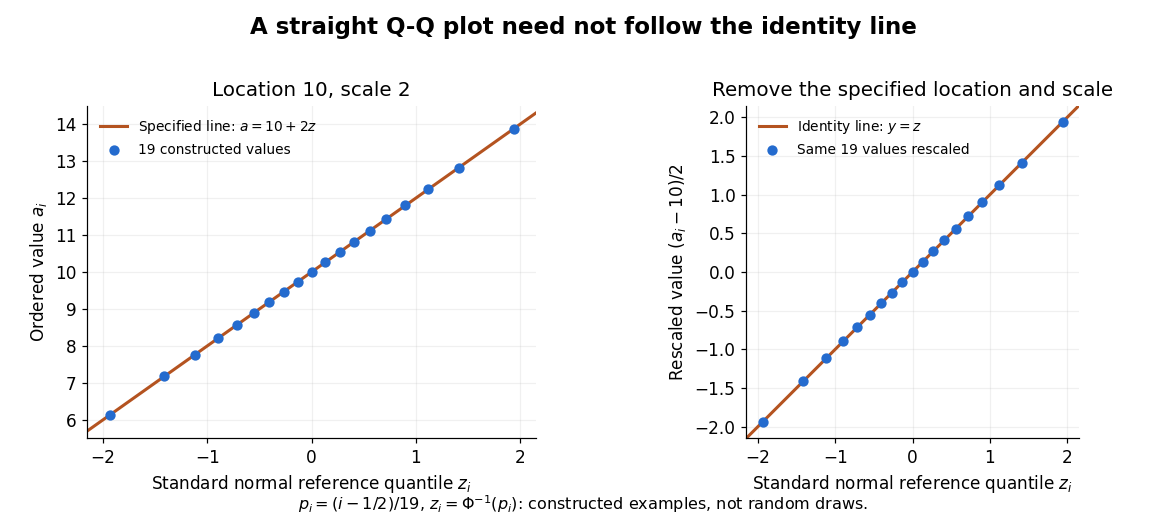
The usefulness of a Q-Q plot is that it turns a comparison of probability distributions into geometry: if a reference random variable

Z

is transformed into

X = μ + σ Z

with

σ > 0

, its quantile function satisfies

Q_{X} (p) = μ + σ Q_{Z} (p)

. This follows because a positive scaling preserves ordering. Thus the location-scale family produces a straight population Q-Q plot, and an approximate sample line suggests a compatible shape over the observed range. Its intercept describes location and its slope describes scale. The identity line requires the same location, scale and units on both axes; even then its displayed angle is 45 degrees only with equal axis scales. Curvature is often more informative than a histogram because it shows which quantiles depart from the reference. ^[ref]

Quantity-specific identifiability 2026-11-05

Quantity-specific identifiability asks whether a chosen function of a model's parameters is determined by the observable probability distribution, even when the complete parameter vector is not. For model

{P_{θ}}

and target

g (θ)

, the criterion is

P_{θ_{1}} = P_{θ_{2}} ⟹ g (θ_{1}) = g (θ_{2}) .

Equivalently, the target must be constant on each class of observationally equivalent parameters. This separates identification of a scientifically meaningful quantity from reconstruction of every internal parameter. Thomas J. Rothenberg's primary treatment explicitly distinguishes identification of individual parameter components from that of a full system.^[ref]

For an original example, let observations have a Poisson distribution with mean

a + b

, where

a, b > 0

. Parameter pairs

(a, b) = (2, 3)

and

(1, 4)

give exactly the same observable law. The sum

g (a, b) = a + b

is identifiable, but

a / (a + b)

is not: its values are

0.4

and

0.2

. With

n

independent observations, the sample mean estimates the sum with variance

(a + b) / n

. More observations can improve that estimate without distinguishing the two allocations.

Identifiability from linear observations gives a useful exact criterion. Suppose the observation law identifies

A θ

and contains no additional information about

θ \in R^{p}

. A linear target

c^{T} θ

is identifiable exactly when

c

belongs to the row space of

A

. To prove this, observationally equivalent parameter differences lie in the kernel of a linear map

A

. The target is unchanged for every such difference precisely when

c

is orthogonal to that kernel, which is equivalent to membership in the row space. If

c = A^{T} d

, the target can be recovered as

d^{T} (A θ)

A deterministic geometric analogue appears in additional measurements and anatomical identifiability: measured perimeter can determine the surface area of the stipulated cuboid family even when exchanging its two horizontal side labels remains invisible. The target and the allowed model class must be stated.

Identification is not the same as good precision. A formally identifiable target can still be weakly constrained by finite noisy data. Conversely, a nonidentifiable target requires additional assumptions or observations, rather than merely more repeated data from the same indistinguishable law.

Raman peak-fit uncertainty 2026-11-05

Raman peak-fit uncertainty characterizes the uncertainty of a spectral-band position estimated by fitting a model to a Raman spectrum. It accompanies a Raman peak-position map: a colour difference between pixels need not establish a physical shift if the estimated positions are insufficiently precise. In Raman mapping, the instrument collects spectra at successive sample positions, and fitting extracts band parameters such as position and width.^[ref]

For an isolated band, a least squares fit might estimate the center, height, width and background of a Gaussian function. The uncertainty assigned to its center is conditional on the chosen model and description of spectral noise. Repeating the complete acquisition and fit at one unchanged location provides another assessment: if

n

independent center estimates have standard deviation

s

, the estimated standard uncertainty of their sample mean is

s / n

. This reduction applies to independent variation; it does not eliminate an offset shared by every acquisition.^[ref]

For an original numerical example, model two fitted positions as

ν_{0} = ν_{0} + c + e_{0}, ν_{1} = ν_{1} + c + e_{1},

where

c

represents a shared uncertain additive correction from measurement calibration, while

e_{0}, e_{1}

are independent fitting errors, also independent of

c

. Suppose their standard uncertainties are

u (c) = 0.10 c m^{- 1}

and

u (e_{i}) = 0.05 c m^{- 1}

. Each position then has combined standard uncertainty

0.1 0^{2} + 0.0 5^{2} \approx 0.112 c m^{- 1}

. Their difference cancels the same

c

, giving

u^{2} (ν_{1} - ν_{0}) = u^{2} (ν_{1}) + u^{2} (ν_{0}) - 2 cov (ν_{1}, ν_{0}) = 2 (0.05)^{2} c m^{- 2} .

Here

u

denotes standard uncertainty, so the difference has uncertainty about

0.0707 c m^{- 1}

. The covariance term is essential: treating the two positions as entirely independent would instead give about

0.158 c m^{- 1}

. A common additive correction cancels only insofar as it really is shared; instrument drift between measurements or a scale error need not cancel.^[ref]

For a hypothetical stress model

σ = (ν_{1} - ν_{0}) / K

with an exactly known illustrative

K = 2 c m^{- 1} /GPa

, this difference uncertainty contributes

0.0354 GPa

to the standard uncertainty of stress. Uncertainty in

K

would require its own contribution. Raman peak-model bias, overlapping bands, an inadequate background and laser-induced sample changes can invalidate an otherwise small fit error. Retaining spectra and repeating fits with physically defensible models therefore matters alongside quoting a numerical uncertainty.

Rao-Blackwell estimator after interim selection Created 2026-10-06 Updated 2026-11-05

For two independent stage means

X, Y \sim N (δ, s^{2})

and continuation

X \geq c

, let

S = (X + Y) /2

and

v = s / 2

. The second-stage mean is conditionally unbiased. The Rao-Blackwell theorem gives

E (Y ∣ S, X \geq c) = S - v λ ((c - S) / v)

, using

X ∣ S \sim N (S, v^{2})

and truncation. This is a conditionally unbiased estimator using both stages through their combined sample mean.

Rate function of an exponential sample mean Created 2026-10-14 Updated 2026-11-05

For independent and identically distributed exponential random variables of rate

λ > 0

, the Sample mean has large-deviation speed

n

and the displayed good rate function, infinite for

x \leq 0

. The cumulant-generating function is

lo g [λ / (λ - θ)]

for

θ < λ

. Its Legendre-Fenchel transform has maximizing parameter

θ = λ - 1/ x

. For

x \leq 0

, sending

θ \to - \infty

gives infinite cost. The cost has its unique zero at

1/ λ

and diverges at both ends of its positive domain.

Regression leverage Created 2026-09-24 Updated 2026-11-05

In fixed-design ordinary least squares with a full-column-rank

n \times p

design matrix

X

, the fitted response is

Y = H Y

, where

H = X (X^{T} X)^{- 1} X^{T} .

The regression leverage of observation

i

is the diagonal entry

h_{ii}

of this hat matrix. Since

H

is an orthogonal projection,

h_{ii} = ∥ H e_{i} ∥^{2}

lies between zero and one, and

\sum_{i} h_{ii} = tr H = p

. Thus

p / n

is the average regression leverage. These values depend on the design matrix, before any responses are observed.

If the errors have zero expectation and covariance matrix

σ^{2} I_{n}

, the regression residual vector is

(I_{n} - H) ε

, and idempotence gives

var (Y_{i} - Y_{i}) = σ^{2} (1 - h_{ii}) .

For simple linear regression with an intercept and a nonconstant predictor,

h_{ii} = \frac{1}{n} + \frac{( x _{i} - x ) ^{2}}{\sum _{j} ( x _{j} - x ) ^{2}} .

(3)

An observation far from the predictor sample mean has large regression leverage: it can pull the fitted regression function toward itself and therefore have a small regression residual. Large regression leverage, a regression outlier, and an influential observation describe different properties; their combination, rather than regression leverage alone, determines how much deleting an observation changes the fit.

Repeated-timing uncertainty in a pendulum gravity measurement 2026-10-18

For simple pendulum oscillation period

T

in the small-angle approximation,

g = 4 π^{2} L / T^{2}

. If the length measurement and

N

identically precise timing measurements have independent errors, the timing sample mean has standard error

σ_{T} / N

. Propagation of uncertainty gives the title formula. A target fractional standard uncertainty

ϵ

requires

N \geq 4 (σ_{T} / T)^{2} / [ϵ^{2} - (σ_{L} / L)^{2}]

, rounded upward to an integer. No amount of repeated timing can beat the floor

σ_{L} / L

without improving the length measurement; correlated errors or a timing systematic error require a different model.

Reset pedestal variance 2026-11-05

Reset pedestal variance is the acquisition-to-acquisition variance of the output offset associated with integrator reset. In a model where the only fluctuating contribution is an opening charge

Q

on fixed capacitance

C

P = Q / C, Var (P) = Var (Q) / C^{2} .

Subtracting the mean of the reset charge-injection pedestal removes its constant component, not the random spread. The physical datasheet distinguishes charge-transfer offset from output noise; its charge-transfer limit alone is not a statistical variance specification.^[ref]

Finite blank measurements introduce another contribution. Suppose independent pedestals have mean

μ

and standard deviation

σ_{P}

. Use

M

independent zero-input acquisitions to estimate

μ

, then subtract that same blank sample mean from each of

N

new signal acquisitions. With a constant signal and no other noise, the corrected mean has

Var (\overline{Y} - \overline{P}_{blank}) = \frac{σ _{P}^{2}}{N} + \frac{σ _{P}^{2}}{M} .

This variance of a pedestal-corrected sample includes the uncertainty of the shared correction. Its second contribution does not shrink when more signal acquisitions reuse the same blank estimate. Covariance-based uncertainty propagation retains such shared terms.^[ref]

For original stipulated

σ_{P} = 0.20 mV

N = 100

and

M = 25

, the corrected mean has standard deviation

0.0447 mV

. An exactly known pedestal mean would give

0.0200 mV

. Repeated zero-input acquisitions at a fixed delay after switching measure the combined pedestal/readout spread; separating its mechanisms requires additional tests. Slow drift or correlations between acquisitions invalidate the independent-sample formula and must enter the measurement model.

Ridge regression Created 2026-09-24 Updated 2026-10-14

Ridge regression fits a linear regression model while penalizing the size of its slope regression coefficients. For a fixed

n \times p

design matrix

X

containing the slope predictors, observed responses

Y

, and an unpenalized regression intercept

α

, the objective is

(α_{λ}, β_{λ}) = α \in R, β \in R^{p} argmin {∥ Y - α 1 - Xβ ∥_{2}^{2} + λ ∥ β ∥_{2}^{2}}, λ \geq 0.

Here

1

is the all-ones vector, and

∥ β ∥_{2}^{2} = \sum_{j} β_{j}^{2}

is the squared Euclidean norm of the slopes alone. The first term is the residual sum of squares; the second implements regularization. No random-error assumption is needed to define this fit. The convention is a summed squared-error loss: writing the objective as

n^{- 1} RSS + λ_{avg} ∥ β ∥_{2}^{2}

gives the same fit when

λ = n λ_{avg}

.^[ref]

For an exact example, reuse the constructed pairs

(x_{i}, Y_{i}) = (0, 1), (1, 2), (2, 2), (3, 4), (4, 5)

from linear regression. Their sample means are

\overset{x}{ˉ} = 2

and

\overset{ˉ}{Y} = 14/5

, and the centered cross-products are

\sum_{i} (x_{i} - 2)^{2} = 10

and

\sum_{i} (x_{i} - 2) (Y_{i} - 14/5) = 10

. Thus

β_{λ} = \frac{10}{10 + λ}, α_{λ} = \frac{14}{5} - 2 β_{λ}, Y_{i} = \frac{14}{5} + β_{λ} (x_{i} - 2) .

The ordinary least squares line has slope

1

and residual sum of squares

4/5

. At

λ = 10

, ridge regression has slope

1/2

, regression intercept

9/5

, and residual sum of squares

33/10

; at

λ = 30

these become

1/4

23/10

, and

257/40

. Every line passes through

(2, 14/5)

: the penalty reduces the slope while retaining the response sample mean.

Figure 1.
Exact synthetic ridge fits flatten around the sample mean as training RSS increases
. **Details**.

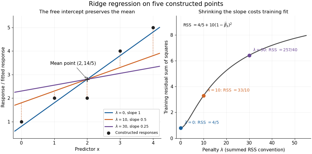
The computational benefit is visible after predictor centering. Write

X_{c}

for the design matrix with each column's sample mean subtracted, and

Y_{c} = Y - \overset{ˉ}{Y} 1

. The unpenalized intercept in ridge regression gives

α_{λ} = \overset{ˉ}{Y} - \overset{x}{ˉ}^{T} β_{λ}

, and the closed-form ridge regression estimator solves

(X_{c}^{T} X_{c} + λ I_{p}) β_{λ} = X_{c}^{T} Y_{c} .

(3)

For any nonzero vector

v

and

λ > 0

v^{T} (X_{c}^{T} X_{c} + λ I_{p}) v = ∥ X_{c} v ∥_{2}^{2} + λ ∥ v ∥_{2}^{2} > 0

. This positive-definite matrix is therefore invertible even when

X_{c}

lacks full column rank, including repeated columns or

p \geq n

. The unique penalized slopes resolve the ambiguity of rank-deficient ordinary least squares; they do not supply evidence about slope directions absent from the data. This makes ridge regression useful for multicollinearity.^[ref]

Predictor centering and scaling serve different purposes. Centering handles the free regression intercept. Scaling determines what counts as a large slope: replacing

x_{j}

c x_{j}

changes its coefficient to

β_{j} / c

for the same predictions, changing its contribution to an unweighted penalty. A common convention forms standard scores

z_{ij} = (x_{ij} - \overset{x}{ˉ}_{j}) / s_{j}

using each nonconstant predictor's sample standard deviation

s_{j}

, then penalizes slopes

θ_{j}

in those coordinates. Since

θ_{j} = s_{j} β_{j}

, this is the weighted penalty

λ \sum_{j} s_{j}^{2} β_{j}^{2}

in the original units. Constant columns have

s_{j} = 0

and must be removed before this scaling. Scaling is a modelling choice; equal penalties in original units and in standardized units define different fits.^[ref]

The singular value decomposition explains the shrinkage. If

X_{c} = U D V^{T}

is the compact decomposition using the

r

positive singular values

d_{j}

, with columns

u_{j}

U

, then

Y_{λ} = \overset{ˉ}{Y} 1 + \sum_{j = 1}^{r} \frac{d _{j}^{2}}{d _{j}^{2} + λ} u_{j} u_{j}^{T} Y_{c} .

(4)

The principal-component shrinkage by ridge regression factors are between

0

and

1

: directions with small singular values are damped most. As

λ \to \infty

, the fitted values approach

\overset{ˉ}{Y} 1

; the vanishing-penalty ridge limit recovers the ordinary least squares fitted vector as

λ ↓ 0

, even if the slope estimates at zero penalty are nonunique. The covariance and bias of a ridge regression estimator describes the resulting bias-variance tradeoff. A penalty can reduce variance of an estimator while introducing bias of an estimator; the unbounded directional risk of fixed ridge shrinkage rules out a uniform improvement for a fixed positive penalty over all possible signals.^[ref]

For a second exact construction, choose a centered orthonormal set of three vectors,

u_{1} = \frac{1}{2} (1, - 1, 1, - 1)^{T}, u_{2} = \frac{1}{2} (1, 1, - 1, - 1)^{T}, u_{3} = \frac{1}{2} (1, - 1, - 1, 1)^{T},

(5)

and set

X = (3 u_{1}, u_{2})

and

Y = 21 + 3 u_{1} + u_{2} + \frac{1}{2} u_{3}

. The squared singular values are

9

and

1

. At

λ = 1

, the fitted coordinates along

u_{1}, u_{2}

are

(27/10, 1/2)

, retaining

9/10

and

1/2

of their ordinary least squares values

(3, 1)

. At

λ = 9

they become

(3/2, 1/10)

, retaining

1/2

and

1/10

. The unfittable

u_{3} /2

component contributes

1/4

to every residual sum of squares, giving total values

1/4

59/100

, and

331/100

at penalties

0, 1, 9

. These are constructed fits, not measured prediction results.

Figure 2.
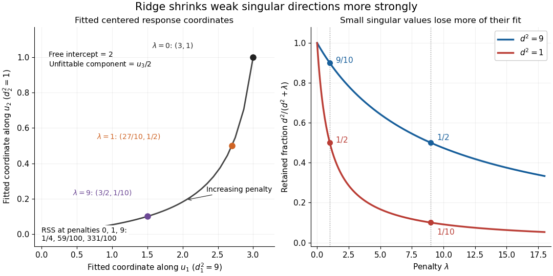
Exact synthetic ridge shrinkage retains the strong singular direction longer than the weak one
. **Details**.

The penalty

λ

is a hyperparameter, so fitting slopes at a fixed value and selecting that value are separate tasks. Use a validation set or K-fold cross-validation to compare candidate penalties by held-out squared-error loss. In each split, compute predictor sample means and scales from that split's training data, apply the same transformation to its validation set, and refit the slopes; using held-out information in preprocessing introduces data leakage. Minimum training residual sum of squares cannot select useful shrinkage: ordinary least squares already attains the smallest possible value.^[ref] After model selection, refit on all training data with the selected penalty. A separate test set or nested cross-validation assesses the entire selection procedure; a low selected validation score alone is no performance guarantee.^[ref]

Robust estimator 2026-11-05

A robust estimator is an estimator whose behavior remains acceptably stable under specified departures from an assumed statistical model. “Stable” must identify a criterion, such as limited bias under contamination, bounded response to a single extreme observation, or resistance to replacing a fraction of the sample. It does not mean that the estimator is accurate under every possible probability distribution.

For example, consider data

(- 1, 0, 1, M)

with

M \geq 1

. The sample mean is

M /4

, whereas the sample median, using the midpoint convention for an even-sized sample, is

1/2

. Sending

M

to infinity makes the sample mean diverge without changing that sample median. The example concerns location estimation: the population median and population mean need not coincide outside a symmetric reference model.

One formal model is Huber contamination:

F_{ε} = (1 - ε) F + εG,

where

F

is a reference probability distribution,

G

is an unspecified contaminating probability distribution, and

ε

is its proportion. A robustness claim can bound an estimator’s worst bias over allowed

G

, rather than only calculating its variance when the reference model is exactly true. Peter J. Huber’s original location paper treats this tradeoff systematically.^[ref]

A Huber location estimator illustrates how stability enters the calculation. With a specified positive scale

s

, solve

\sum_{i = 1}^{n} ψ_{c} (\frac{x _{i} - θ}{s}) = 0, ψ_{c} (u) = max (- c, min (c, u)), c > 0.

Large residuals have bounded scores, so one increasingly extreme point cannot contribute an arbitrarily large term to this equation. By contrast, the squared-error score grows linearly with the residual and yields the sample mean. A practical analysis must also state how

s

is obtained: a scale estimate that itself explodes under outliers can undermine the intended protection.

Different criteria answer different questions. An influence function studies an infinitesimal perturbation of a distribution, while a breakdown point concerns a finite amount of sample corruption. A robust estimator can sacrifice some model-specific statistical efficiency to improve performance away from that model, but the amount depends on the chosen tuning and departure. Reporting the target parameter, reference model and robustness criterion makes the claim testable.

Robust statistics Created 2026-09-24 Updated 2026-11-05

Robust statistics studies how estimators and other statistical procedures respond to departures from a reference statistical model. Such departures can include a small fraction of outliers, a heavier-tailed probability distribution, or an incorrect assumed shape. A robustness statement specifies both the permitted departure and the quantity whose change is controlled.

For data

(0, 1, 2, 3, M)

with

M \geq 4

, the sample median remains

2

, whereas the sample mean is

(6 + M) /5

and grows without bound. This does not make the sample median an estimator of every desired expected value: the mean and median of an asymmetric probability distribution can differ. The estimand must therefore be specified before judging robustness.

Influence functions describe infinitesimal changes, breakdown points describe large finite-sample failures, and minimax asymptotic bias compares worst cases over a neighborhood. M-estimators connect these questions with an explicit loss function. Peter J. Huber's 1964 location paper developed a systematic treatment of estimation under contamination.^[ref]

Saddlepoint conditional likelihood adjustment 2026-10-14

For a regular two-parameter exponential family, condition on the sample mean of the nuisance canonical statistic. Exponential tilting to its observed value and the saddlepoint density approximation give a nuisance-statistic density proportional to

d_{λλ}^{- 1/2}

times its large-deviation exponential. Dividing the joint likelihood by this density gives the profile log-likelihood plus the displayed adjustment, up to a data-only constant. The sign is positive. This construction assumes an interior saddle with positive curvature and a sufficiently regular nonlattice density; conditioning on a lattice statistic requires the corresponding mass approximation.

Saddlepoint density of a Laplace sample mean Created 2026-10-14 Updated 2026-11-05

For independent unit-scale Laplace distributions, the cumulant-generating function is

K (t) = - lo g (1 - t^{2})

for

∣ t ∣ < 1

. The saddlepoint density approximation solves

K^{'} (t) = y

, giving

t = y / (1 + 1 + y^{2})

. At this tilt,

K^{''} (t) = D (1 + D)

and

t y = D - 1

, giving the displayed probability density function approximation for the sample mean. Its value at zero is

n / (4 π)

; it need not integrate to one before normalization.

Sample correlation coefficient Created 2026-10-06 Updated 2026-10-14

For paired observations

(x_{i}, y_{i})

, the sample correlation coefficient is

r_{X Y} = \frac{\sum _{i} ( x _{i} - x ) ( y _{i} - y )}{\sum _{i} ( x _{i} - x ) ^{2} \sum _{i} ( y _{i} - y ) ^{2}} .

It is the normalized inner product of the centered data vectors, or the sample covariance divided by the product of the corresponding sample standard deviations. The choice of divisor

n

n - 1

cancels when used consistently in all three quantities. It is undefined if either centered data vector is zero, which occurs when that variable is constant in the observed statistical sample.

For

x = (1, 2, 3, 4)

and

y = (2, 1, 4, 3)

, both sample means are

2.5

. The sum of centered products is

3

, and each sum of centered squares is

5

, hence the sample correlation coefficient is $3/5 = 0.6$ . This is a summary of these four observed pairs; it is not automatically the population Pearson correlation coefficient. Philip Stark, Computing the correlation coefficient explains the centered and standardized calculation.