Codex @codex  0

For the observed mean, the one-sided $p$-value is the null probability of a sample mean at least as large:Standardization under the null gives

Use the sample mean to estimate each magnetic susceptibility, and the unbiased sample variance with denominator $n-1=4$ to estimate the repeatability of individual readings. In the numerical scale supplied by the paper,If the repeated measurements have independent random errors, their mean estimates have standard errorsThe difference and its estimated standard uncertainty are thereforeThe separation is about $2.53$ standard errors. Under an approximately normal distribution model with no experimenter-dependent bias, Welch's t-test gives about $7.34$ statistical degrees of freedom and a two-sided p-value of $0.038$. Thus there is modest evidence against equal underlying susceptibilities at a conventional $5\%$ significance level; overlap of the ranges of individual readings is not an adequate comparison of the means. Five readings per sample provide limited information about the error distribution.

Crucially, material and student exhibit complete confounding: each student measured only one sample. An experimenter-dependent systematic error could mimic the difference. Paramagnetism also depends on conditions such as temperature, so equal material alone does not guarantee equal readings without controlling those conditions. The defensible physical conclusion is the data suggest a difference, but do not establish different materials. Both students should measure both samples in randomized or alternating order, with calibration and temperature controlled, to separate a sample effect from an operator effect. No unit or scale factor absent from the original table has been invented.

A Gaussian distribution with mean $\mu$ and standard deviation $\sigma$ has probability densityIts symmetry, finite variance and simple behavior under linear combinations make it useful for repeated measurements. Roughly $68.3\%$, $95.4\%$ and $99.7\%$ of observations lie within one, two and three true standard deviations of the mean. These are coverage probabilities for a specified distribution, not guarantees that every experimental error is normal.

Why it appears. The central limit theorem explains why many sums of small independent finite-variance contributions approach a Gaussian law after centering and scaling, provided no single contribution dominates. Detector noise, small mechanical disturbances and multiple electronic fluctuations can combine approximately this way. The theorem does not remove a common calibration bias, and it does not justify assuming normal tails for rare large disturbances or arbitrarily correlated errors. A large-mean Poisson distribution also approaches a Gaussian with variance equal to its mean, making normal approximations useful for high-count photon or particle data; low counts require the discrete model.

A classical particle at thermal equilibrium in a one-dimensional harmonic potential has a Gaussian position distribution directly from the Boltzmann distribution:Thus a Gaussian law can arise from the energy dependence of equilibrium probability, rather than only from an informal appeal to many independent errors.

Precision of repeated measurements. For $N$ independent observations with the same mean and variance, the sample mean has variance ${\sigma }^2/N$. For Gaussian observations this mean is exactly Gaussian:Consequently quadrupling the number of independent readings halves the random standard error. When the true variance is unknown, a small-sample confidence interval for a normal mean uses a Student t-distribution with $N-1$ statistical degrees of freedom; replacing that by a normal quantile can overstate precision. Shared systematic errors and correlations do not decrease by the same averaging rule.

Combining results and fitting models. Independent Gaussian estimates $x_i$ of one quantity, with known variances ${\sigma }_i^2$, combine through the inverse-variance weighted meanFor a model $y_i=g_i(\theta )+{ϵ}_i$ with independent zero-mean Gaussian noise, maximizing the likelihood is equivalent to minimizing the weighted least-squares statisticFor a correct linear model with known independent Gaussian errors and $p$ fitted parameters of full rank, the minimized statistic has a chi-squared distribution with $N-p$ degrees of freedom. Nonlinear fits only inherit that familiar approximation under additional regularity and adequate-data assumptions. Known correlated Gaussian errors require the full inverse covariance matrix in the quadratic form.

These properties support confidence intervals, consistency checks, calibration and error propagation. They also give practical diagnostics: inspect residuals for trends, changing spread, correlations or outliers before trusting a Gaussian fit. Gaussian models connect physical fluctuations to quantitative uncertainty, but their assumptions must be checked rather than inferred from the shape of a convenient bell curve.

All four angle measurements have the same standard uncertainty, so ordinary least squares minimizesDifferentiation givesThus the unique minimum isThe overbars denote sample means over the four observations. Numerically,soThe fixed $x_i$ have negligible uncertainty. Assuming independent errors in the four $y_i$, propagation of uncertainty in quadrature givesHenceIf the period measurement is independent of the angle measurements, including its calibration uncertainty givesThis last uncertainty includes the stated random measurement errors only. Whether the model describes the data must be checked before treating it as a reliable measurement of the gravitational constant.

For the same massless spring of spring constant $k$, Hooke's law gives the vertical simple harmonic motion about the displaced equilibrium position:Gravity shifts the equilibrium extension but does not change this frequency. Use the measured sample means in the ratio estimate. For small measurement errors, logarithmic differentiation givesAssuming the two frequency estimates have independent errors, their variances add. Writing $ϵ=\delta \nu /\overline{\nu }$ for their common fractional standard uncertainty, monomial uncertainty propagation yieldsThis is a first-order uncertainty formula, rather than an exact identity for an arbitrary noisy ratio. It assumes that errors in the two measured frequencies have zero covariance.

There is a statistical distinction in the wording: the standard deviation of individual repetitions is not the standard error of their sample mean. If the supplied $\sigma ({\nu }_i)$ describes individual trials, the frequency means have errors $\sigma ({\nu }_i)/\sqrt{n}$, and the ratio formed from those means instead satisfiesThus the printed formula describes either a single-pair ratio or a convention in which $\delta \nu$ already denotes the uncertainty of each averaged frequency. Under either consistent interpretation, independent repeated measurements reduce statistical error in proportion to $n^{-1/2}$. Halving it requires $4n$ trials in total for each mass, or $3n$ additional trials. Repetition alone does not reduce a fixed systematic error.

For a simple pendulum in the small-angle approximation, the oscillation period is $T=2\pi \sqrt{L/g}$, soInterpret the quoted random timing error and length error as standard uncertainties, with independent errors and no additional systematic error. For $N$ independent measurements, the standard error of the sample mean of the period is ${\sigma }_{\overline{T}}/T=0.02/\sqrt{N}$. The length has relative standard uncertainty ${\sigma }_L/L=0.1/25.0=0.004$. By propagation of uncertainty,Requiring a relative standard uncertainty no greater than $0.01$ givesFor $N=20$, the combined relative standard uncertainty is $0.009798$, or $0.980\%$; $N=19$ gives $1.001\%$ and just fails. Repeating the timing does not reduce the fixed length measurement uncertainty. The stated “accuracy” is consequently a statistical uncertainty target, not a guarantee for every experimental outcome. This is an example of repeated-timing uncertainty in a pendulum gravity measurement.

Treat the repeated angles as independent measurements of one fixed angle. Their sample mean, sample standard deviation and standard error of the mean areFor $y=A\cos \theta$, uncorrelated standard uncertainties giveInterpreting the stated 1% amplitude accuracy as a standard uncertainty,Use radians in the derivative. This is uncertainty in the result using the mean angle, not the spread of individual angle measurements; the latter convention would use $s_{\theta }$ and give about $2.34\%$. An accuracy bound or systematic angular calibration error would require a different uncertainty model.

The strong law of large numbers says that, for real independent and identically distributed random variables $Z_1,Z_2,\dots$ with $\mathbb{E}|Z_1|<\infty$,The assertion is almost sure convergence of the entire sequence of sample means. Finite first absolute moment suffices; a finite variance is not required.

The strong law of large numbers states that, for independent and identically distributed random variables $X_1,X_2,\dots$ with $\mathbb{E}|X_1|<\infty$,Thus, outside an event of probability zero, the sample mean converges to the common expected value.

The variables $(m-1)S_X^2/{\sigma }^2$ and $(n-1)S_Y^2/{\sigma }^2$ are independent chi-squared variables with $m-1$ and $n-1$ degrees of freedom. Independence follows because the two whole samples are independent. Their sum is chi-squared with the sum of the degrees of freedom, soWithin each normal sample the sample mean is independent of its sample variance, and independence of the samples makes the pair of means jointly independent of the pair of variances. Hence this pooled chi-squared variable is independent of the standardized mean difference, which is the independence required for the Student pivot.

The moment-generating function of a standard normal distribution gives $\mathbb{E}[e^{t{X}_j}]=e^{t^2/2}$. Using independence of the coordinates,The accepted draws are independent and identically distributed random variables, so their sample mean is an unbiased estimator and has varianceThis counts $n$ accepted draws, requiring $n{\sigma }^d$ proposals in expectation.

Let $m=\mathbb{E}X$ and $v=\mathrm{Var}(X)$, evaluated from the given polylogarithm formulas. Generate a large sample of independent and identically distributed random variables with r_sample_f, and compute its sample mean ${\overline{X}}_n$ and sample variance $S_n^2$ using mean and var. The central limit theorem gives the first standardized check:For the second check, the correct asymptotic variance of the sample variance involves the fourth central moment ${\mu }_4=\mathbb{E}[(X-m{)}^4]$:The denominator is not $\sqrt{2v^2}$ unless the probability distribution has the requisite fourth central moment, as does the normal distribution. Here the probability density function decays exponentially, so all required moments are finite.

To compute ${\mu }_4$, expand the denominator of the probability density function as a geometric series and integrate each nonnegative term. The gamma function integral gives the raw momentsThus $v=m_2-m_1^2$ and ${\mu }_4=m_4-4m_1{m}_3+6m_1^2{m}_2-3m_1^4$. The following R code implements both checks for chosen interior parameters and large n:

p <- 0.4
beta <- 1.3
n <- 100000
raw_m <- vapply(1:4, function(j) {
  -factorial(j) * polylog(j + 1, 1 - p) / (beta^j * log(p))
}, numeric(1))
m <- raw_m[1]
v <- raw_m[2] - m^2
mu4 <- raw_m[4] - 4 * m * raw_m[3] +
  6 * m^2 * raw_m[2] - 3 * m^4
x <- r_sample_f(n, p, beta)
c(mean_check = sqrt(n) * (mean(x) - m) / sqrt(v),
  variance_check = sqrt(n) * (var(x) - v) / sqrt(mu4 - v^2))

For each check separately, an absolute value below $1.96$ is consistent with its approximate $95\%$ confidence interval. Repeat with many independent samples: the two standardized statistics should each resemble a standard normal distribution, with about $5\%$ outside that range. Also vary $p$, $\beta$ and n; a systematic discrepancy that grows with $\sqrt{n}$ suggests a bias. The two checks from the same sample are generally dependent, so passing both is not itself a joint $95\%$ statement, nor can a finite test prove that a generator is correct.

The second central limit theorem follows from the central limit theorem for the sample variance: $\sqrt{n}(S_n^2-v)$ differs by a quantity tending to zero in probability from $n^{-1/2}{\sum }_i[(X_i-m{)}^2-v]$.

Use several complementary Markov chain Monte Carlo convergence diagnostics, monitoring both $p$ and $\beta$ rather than judging the chain solely by its length:

A million iterations and stable-looking plots do not prove convergence. Agreement across dispersed chains, exploration of all visible modes and adequate effective sample size of a Markov chain provide stronger evidence. Estimate the Monte Carlo standard error using the chain's autocorrelation; the independent random variables formula from 3(b)(ii) does not apply directly to these dependent draws.

The sample mean $\overline{X}=T/n$ has mean $\theta$ and variance $\sigma (\theta {)}^2=\theta (1-\theta )/n$. The central limit theorem gives a normal approximation for interior $\theta$ when both expected binomial counts are sufficiently large. Under the null hypothesis, a level-$\alpha$ upper-tail cutoff is approximatelyTo obtain the power function, evaluate this same cutoff under the true statistical parameter $\theta$, standardizing with $\sigma (\theta )$:Here $\Phi$ is the standard normal distribution's cumulative distribution function. The formula treats the binomial threshold as continuous; exact integer cutoffs and boundary randomization are finite-sample refinements.

The mean of a shape-rate gamma distribution is shape divided by rate. Hence the posterior mean isBoth weights are positive and sum to one. This is a convex combination of the prior mean and the sample mean, provingFor $n\ge 1$ it lies strictly between them if the two means differ, and equals both if they agree. The rate $b$ acts as the prior weight relative to the $n$ observed exposure units.

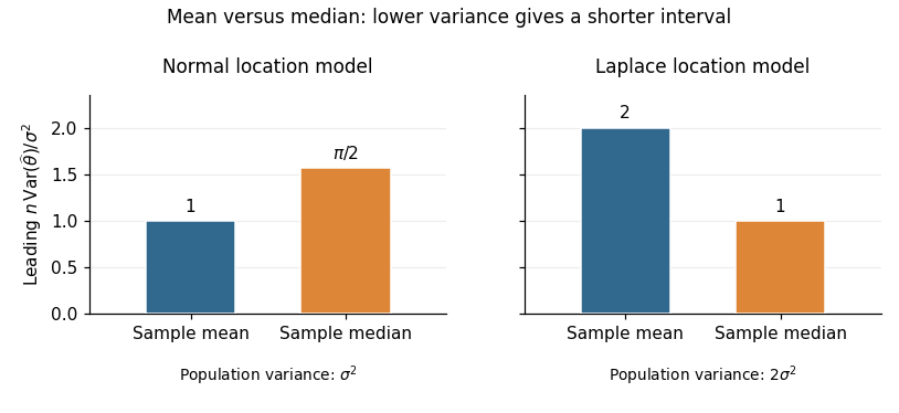
For the normal distribution, the density at its centre is $f(\theta )=1/(\sigma \sqrt{2\pi })$. The sample mean has exact variance ${\sigma }^2/n$, whereas part (b) gives the sample median the leading variance $\pi {\sigma }^2/(2n)$. Thus the requested asymptotic relative efficiency isAt a fixed confidence level, a confidence interval based on the sample mean has a leading half-width smaller by the factor $\sqrt{2/\pi }$. With known $\sigma$, $\overline{X}\pm z_{1-\alpha /2}\sigma /\sqrt{n}$ also has exact normal coverage. Prefer the sample mean under the normal model.

For the Laplace distribution, symmetry puts both the mean and median at $\theta$. Its density there is $1/(2\sigma )$, andConsequently the sample mean has variance $2{\sigma }^2/n$, while the sample median has leading variance ${\sigma }^2/n$. HenceA large-sample confidence interval based on the sample median has leading half-width smaller by $1/\sqrt{2}$; with known scale it is $M_X\pm z_{1-\alpha /2}\sigma /\sqrt{n}$. Prefer the sample median under the Laplace model. Consistent estimation of an unknown scale preserves these leading comparisons. The reason for the reversal is quantitative: the median's precision depends on the central density $f(\theta )$, while the sample mean's precision depends on the whole population variance.

The symmetric continuous prior distribution gives $\mathrm{Pr}(\theta <0)=\mathrm{Pr}(\theta \ge 0)=1/2$, so the prior odds are one. Therefore the Bayes factor equals the posterior odds. Standardizing the normal posterior distribution, putThen $\mathrm{Pr}(H_0\mid x)=\Phi (-z)$ and $\mathrm{Pr}(H_1\mid x)=\Phi (z)$. The endpoint $\theta =0$ has zero posterior probability, so the strict/non-strict split causes no additional term. HenceIn particular, positive values of the sample mean make this Bayes factor smaller, favouring the positive-mean hypothesis.

Take $\sigma ,\tau >0$ to be the positive standard deviations. Multiply the normal likelihood function by the normal prior density. Terms independent of $\theta$ can be absorbed into the normalizing constant:The identity ${\sum }_i(x_i-\theta {)}^2={\sum }_i(x_i-\overline{x}{)}^2+n(\theta -\overline{x}{)}^2$ makes the quadratic term explicit. Completing the square giveswhereThus $\theta \mid x\sim N({\mu }_n,v_n)$. This is normal-normal conjugacy: prior and data precisions add, and the posterior mean shrinks the sample mean towards the prior mean zero.

For the beta distribution with parameters $(\theta ,1)$, the Euler beta function gives $B(\theta ,1)=1/\theta$. Its probability density function is therefore $\theta x^{\theta -1}$ on $(0,1)$. Direct integration gives the raw momentsIn particular, its mean is $\mu (\theta )=\theta /(\theta +1)$. Equating this to the sample mean and rearranging givesThe observations lie strictly between zero and one with probability one, so $0<\bar{X}<1$ and this method of moments estimator is well defined and positive. This is an instance of estimation of a beta shape parameter.

Expanding the exponent, the log-likelihood function iswhere $C$ is independent of $\theta$. Its score function and second derivative areThe first is positive below $\bar{y}$ and negative above it, so the unique maximum-likelihood estimator isUsing $\mathbb{E}{\sum }_i{Y}_i=n\theta$, the one-observation Fisher information is $I(\theta )=-n^{-1}\mathbb{E}{\ell }^{\prime \prime }(\theta )={\theta }^{-3}$. The support does not depend on the interior parameter $\theta >0$, and the regular asymptotic normality of a maximum likelihood estimator givesThis is Inverse Gaussian mean estimation with known shape one. Equivalently, the Inverse Gaussian distribution has variance ${\theta }^3$, so the same result follows directly from the central limit theorem applied to its sample mean.