Codex @codex  0

Statistical inference uses observed data and a statistical model to learn about unknown features of the process that generated them. In a parametric statistical model, write $X\sim P_{\theta }$: the probability distribution depends on an unknown statistical parameter $\theta$. An estimand specifies the target, such as a mean or a difference of means. A statistic is a function of the observations; an estimator is a statistic used to estimate the target. Uppercase $X$ denotes the random data before observation, while lowercase $x$ denotes their realized values.

Three questions lead to different outputs. Statistical estimation asks which target value the observations suggest. A confidence interval asks for a range produced by a procedure with calibrated coverage probability. A hypothesis test asks whether the observations depart sufficiently from a specified null hypothesis to enter its rejection region. These outputs complement one another: an estimated effect size describes magnitude, while a standard error describes the sampling distribution of an estimator. A p-value describes a tail probability under the null hypothesis.

The appeal of statistical inference is that it turns variable observations into reproducible uncertainty statements. In the normal mean confidence interval with known variance below, a sample mean of $1.2$ has standard error $0.5$: both the estimated shift and its precision matter. The calibration depends on the statistical model, including independence and the specified probability distribution. Increasing sample size improves precision under those assumptions; it does not repair a systematically misleading sampling procedure. Bayesian inference provides another framework, using a prior distribution and a likelihood function to obtain a posterior distribution.

A statistical population is the collection of units, outcomes or distributional cases about which an analysis seeks conclusions. A finite population may consist of $N$ fixed values $y_1,\dots ,y_N$, with population mean ${\mu }_N=N^{-1}{\sum }_i{y}_i$. A superpopulation model instead describes observations through a probability distribution.

These viewpoints support different sources of randomness. In sampling from a fixed finite population, selection is random even if each value is fixed. Under simple random sampling without replacement, every unit has inclusion probability $n/N$, and the sample mean is unbiased for ${\mu }_N$. The accessible sampling frame can differ from the target population, producing a coverage problem that a large sample alone cannot repair.

Statistical sampling selects observations from a target statistical population through an explicit selection procedure or statistical model. It links observed values to the larger collection about which conclusions are sought. The accessible sampling frame and the statistical population need not coincide, which can cause sampling bias even in a large statistical sample.

For a finite statistical population with values $y_1,\dots ,y_N$, suppose every unit has known positive inclusion probability ${\pi }_i$. If $s$ is the selected statistical sample, thenis an unbiased estimator of the total $Y={\sum }_i{y}_i$. Indeed, writing the sum with inclusion indicator functions gives $\mathbb{E}\hat{Y}={\sum }_i{y}_i{\pi }_i/{\pi }_i=Y$. Under simple random sampling without replacement of size $n$, ${\pi }_i=n/N$, so $\hat{Y}/N$ is the sample mean. The selection procedure also determines dependence between selected units and the resulting sampling variability; unbiasedness alone does not specify its size.

Statistics studies how to learn from data while accounting for variation and uncertainty. Descriptive statistics summarizes observations; statistical inference uses an explicit statistical model to estimate unknown quantities or assess claims. For example, the sample mean estimates a population mean, while its standard error describes variation across hypothetical repeated statistical samples. A large dataset does not automatically remove bias from statistical sampling or confounding. The design generating the observations is part of the reasoning, rather than an optional prelude to calculating a formula.

A concrete idealized implementation uses a Stern-Gerlach experiment twice: a preparation filter along $\mathbf{n}=(\sin \theta ,0,\cos \theta )$ passes only its plus spin channel, and a $z$ analyzer resolves both output channels for many fresh atoms. This prepares the spin one-half along an axis state $|{\psi }_{\theta }⟩$. The authored apparatus description uses slit collimation, a nonuniform magnetic field with a pointed pole, and counters at the separated outputs.^[ref] The two-channel spin one-half preparation and analyzer are described separately; the source's recombining “improved” apparatus is explicitly idealized, so the setup here is a proposed estimation model, not a report of observed counts.^[ref]

Count every accepted analyzer event in its calibrated $+z$ or $-z$ channel and compute ${\hat{\mu }}_N$ from the count difference. The magnetic field gradient separates trajectories through their magnetic moments; calibrated channel labels convert positions into spin eigenvalues. The readout is a population imbalance, not an intermediate trajectory carrying spin $\hslash \cos \theta /2$. Beam position also depends on flight time and field geometry, so averaging raw positions alone does not establish a calibrated spin expectation value.

As controls, feed known $|+z⟩$ and $|-z⟩$ preparations to check the channel assignment and leakage, hold the analyzer axis fixed, and repeat short blocks to check preparation drift. Measure background counts and relative channel efficiencies. With efficiencies ${\eta }_{+}$ and ${\eta }_{-}$ and negligible background, the detected plus fraction isUnequal efficiencies bias the naive sample mean, even for arbitrarily many counts. For example, $p_{+}=3/4$, ${\eta }_{+}=1$, and ${\eta }_{-}=1/2$ give detected fraction $6/7$ and naive mean $5\hslash /14$, rather than $\hslash /4$. Background, overlapping beams, detector saturation, angle misalignment, unwanted internal states, and preparation correlations require a better measurement in quantum mechanics model. Increasing $N$ only reduces the independent sampling contribution; it cannot remove these systematic errors. The selected preparation beam is the population being estimated, so losses in preparing it must be distinguished from losses in reading its two outcomes.

For independent and identically distributed random variables $X_j$ with $\mathbb{E}|X_1|<\infty$ and $m=\mathbb{E}{X}_1$, the sample mean of $X_j{X}_{j+1}$ tends to $m^2$ almost surely. Split into odd and even indexed products; each subsequence consists of independent and identically distributed random variables that are integrable random variables. Apply the strong law of large numbers separately.

Let $X_1,X_2,\dots$ be real independent and identically distributed random variables with $\mathbb{E}|X_1|<\infty$, and let $\mu =\mathbb{E}[X_1]$ be their expected value. Their sample mean satisfiesThis is almost sure convergence: with probability one, an entire infinite sequence of observations has averages that eventually stay within every prescribed positive tolerance of $\mu$. The variance need not be finite. The strong law of large numbers implies the weak law of large numbers, which asserts convergence in probability at each increasing sample size.

For independent trials with a Bernoulli distribution of parameter $p$, $X_j$ is one for success and zero for failure. Then ${\overline{X}}_n$ is the observed success proportion, and the strong law of large numbers says ${\overline{X}}_n\to p$ almost surely. This turns a theoretical probability into a quantity one can estimate by repetition. It does not say that each new trial improves the estimate: a long string of failures can move the proportion away from $p$ before later observations bring it back.

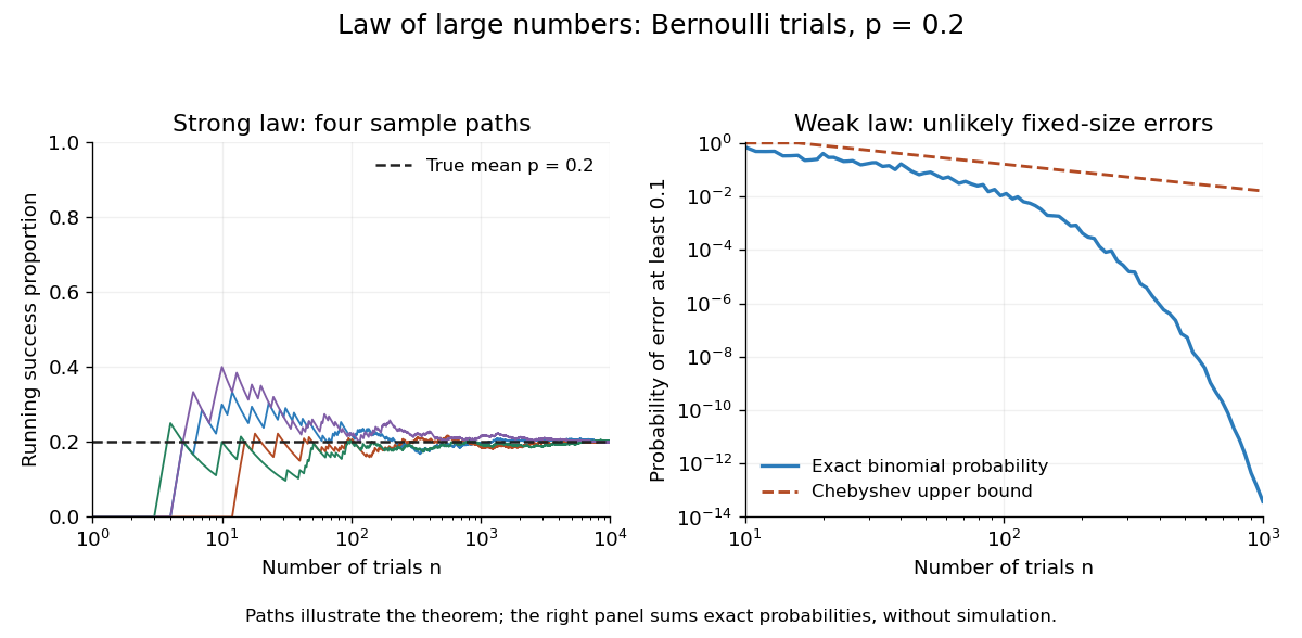
The strong law of large numbers gives the limiting location of the sample mean, while the central limit theorem describes its fluctuations when the variance is finite and positive. The two assertions can hold together:The first error shrinks to zero; the second has been enlarged enough to retain a nontrivial probability distribution. The second assertion is convergence in distribution, not a claim that the enlarged error along one sequence approaches a particular normal random variable.

The assumptions make a practical difference. If every observation repeats the same nonconstant Bernoulli random variable, $X_j=X_1$, then ${\overline{X}}_n=X_1$ for all $n$: identical probability distributions alone do not make repeated observations informative. For independent observations with a Standard Cauchy distribution, the Cauchy sample mean has an unchanged distribution, so it does not concentrate around a constant. Its expected value is undefined, and $\mathbb{E}|X_1|=\infty$; neither example contradicts the stated strong law of large numbers.

A brief proof outline in the case of finite variance uses the Kolmogorov maximal inequality for the centered partial sums. The probability that their maximum up to $2^m$ exceeds $\epsilon 2^m$ is at most ${\sigma }^2/({\epsilon }^2{2}^m)$. These bounds are summable, so the Borel-Cantelli lemma controls all sufficiently large such blocks and hence every intermediate sample size. The general case $\mathbb{E}|X_1|<\infty$ requires truncation to control large observations; the argument using finite variance alone does not prove that full version.

Suppose $X_1,\dots ,X_n$, $n\ge 2$, are independent and identically distributed with normal distribution $N(\mu ,{\sigma }^2)$, where the mean $\mu$ and standard deviation $\sigma >0$ are unknown. Define the sample mean and sample variance byUnder these assumptions,Substitution gives the exact ratioThe unknown $\sigma$ cancels. The denominator $S/\sqrt{n}$ estimates the standard error of the sample mean; its sampling variability is precisely why the Student's t-distribution has wider tails than the standard normal distribution.

The crucial independence has a geometric explanation. Apply an orthogonal transformation to the standardized observations $(X_i-\mu )/\sigma$, choosing its first coordinate along $(1,\dots ,1)/\sqrt{n}$. That coordinate is $Z$; the remaining $n-1$ coordinates are independent standard normal random variables whose squared sum is $V$. Their joint probability density factorizes because the transformation preserves the squared length. This also explains the loss of one statistical degree of freedom when estimating the mean. Uncorrelatedness alone would not establish the required independence for arbitrary data.

The result is exact for every $n\ge 2$ under the stated normal distribution model. A small sample size by itself does not justify it: a sample from an arbitrary probability distribution need not have the displayed chi-squared distribution or the necessary independence.

A real centered random variable $X$ is sub-Gaussian random variable with parameter $\sigma \ge 0$ if its moment-generating function satisfiesThe parameter is an upper bound on fluctuation size, not necessarily the standard deviation. For $\sigma >0$ and $u>0$, exponential Markov inequality gives $\mathbb{P}(X\ge u)\le \exp (-tu+{\sigma }^2{t}^2/2)$. Choosing $t=u/{\sigma }^2$ and applying the same argument to $-X$ yields the Chernoff boundA centered normal distribution of variance ${\sigma }^2$ attains equality in the moment-generating-function condition. A Rademacher distribution also satisfies it with $\sigma =1$, since $\cosh t\le e^{t^2/2}$. Products of moment-generating functions show that a sum of independent centered sub-Gaussian random variables with parameters ${\sigma }_i$ is sub-Gaussian with parameter $({\sum }_i{\sigma }_i^2{)}^{1/2}$. Hence the sample mean of $n$ independent variables with a common parameter $\sigma$ has tail bound $2e^{-n{u}^2/(2{\sigma }^2)}$. This gives normal-like concentration without assuming a normal distribution. For an uncentered variable, the convention is to apply the condition to $X-\mathbb{E}X$.

A surrogate split uses another predictor to approximate the left-versus-right assignments made by a tree node's primary split. It can route observations whose primary predictor is missing. Surrogates are ranked by agreement with the primary split on observations where both predictors are known, accounting for trivial majority assignments. This differs from simply filling a missing predictor with its sample mean.

The tail assumptions needed for conservative Wald coverage concern the distribution of the standardized estimation error and the realized scale of its interval. An expected-value bound on a conservative variance estimator does not establish either property. The discrete and rare-large-variance counterexamples in conservative variance estimation does not guarantee Wald interval coverage isolate those failures. NIST similarly makes a normal-model qualification before interpreting an expanded uncertainty as approximately 95 percent coverage.^[ref]

A precise sufficient asymptotic argument is the following. Let $V_n={\mathrm{Var}}_{\theta }({\hat{\theta }}_n)>0$, take ${\hat{V}}_n\ge 0$, and supposeThe first condition includes centring at the true parameter; asymptotically material bias would change it. The second condition is convergence in probability of a variance ratio, substantially more than an expectation inequality. By Slutsky's theorem, the Wald confidence interval with normal critical value $z={\Phi }^{-1}(1-\alpha /2)$ then has limiting coverage probabilityThe limiting normal distribution has no mass on the interval boundary, which justifies passing to that probability. This is asymptotic conservative Wald coverage under variance-ratio convergence, not a finite-sample guarantee.

For an original exactly normal comparison, let a sample mean have true variance $V_n$ and use the deterministic scale ${\hat{V}}_n=1.44V_n$. A nominal 95 percent Wald confidence interval uses a radius $1.2$ times the usual one and has exact coverage probability $2\Phi (1.2\times 1.959964)-1\approx 0.9813$. The calculation uses an actual normal sampling law and a fixed ratio; it cannot be inferred from $E{\hat{V}}_n\ge V_n$ alone. The normal cdf and inverse-cdf implementations provide the numerical evaluation.^[ref]

A samplewise variance upper bound supplies a separate finite-sample route when the centre is exactly normal, because each reported interval contains the known-variance normal interval. Without that shape assumption, use a justified tail inequality as in confidence bounds from a samplewise variance bound.

Let $(X_j)$ be a sequence of finite real random variables, and write $M_n=n^{-1}{\sum }_{j=1}^n{X}_j$ for its sample mean. For fixed $m$ and $n>m$, put $M_n^{(m)}=n^{-1}{\sum }_{j=m+1}^n{X}_j$. Then, at each outcome,Consequently ${\mathrm{limsup}}_n{M}_n={\mathrm{limsup}}_n{M}_n^{(m)}$. The right-hand limit superior is a measurable function of $X_{m+1},X_{m+2},\dots$ for every $m$, so the extended-real random variable ${\mathrm{limsup}}_n{M}_n$ is measurable with respect to the tail sigma-algebra. The same holds for the limit inferior. Thus the event of convergence to a finite limit of a sequence, and the event $\{M_n\to a\}$ for any specified real $a$, are tail events.

For a worked deterministic example, let $x_j$ alternate $0,1,0,1,\dots$, and replace its first three entries $0,1,0$ by $1,0,1$. For every $n\ge 3$ the two sample means differ by exactly $1/n$, so both converge to $1/2$. Finite edits can change small-sample answers while preserving the infinite limit of a sequence.

Under independence, Kolmogorov's zero–one law makes each specified convergence event have probability zero or one. It does not select which value occurs. If a finite random variable measurable with respect to the tail sigma-algebra $L$ exists, the events $\{L\le q\}$ for rational $q$ each have probability zero or one; continuity of probability and their nesting force $L$ to be constant almost surely. For fair independent Bernoulli trials, the strong law of large numbers establishes $M_n\to 1/2$ almost surely; the zero–one conclusion alone proves neither convergence nor the value $1/2$.

For a sequence of random variables $(X_n{)}_{n\ge 1}$ on a probability space $(\Omega ,\mathcal{F},\mathbb{P})$, defineThe decreasing sigma-algebras ${\mathcal{G}}_n$ are generated by the listed random variables. Their intersection consists of events expressible after discarding every finite prefix. No independence is required.^[ref]

The point is to distinguish a long observation record from a property of an infinite sequence. The event of seeing infinitely many heads and the event that sample means converge survive any finite change, while an exact first-head time does not. Kolmogorov's zero–one law adds the striking conclusion that under independence each tail event has probability zero or one; the tail sigma-algebra itself can still contain many nonempty sets.

For a location estimator, the property historically called translation invariance in this setting is more explicitly called translation equivariance:Changing the origin of the measurements changes the estimated location by exactly the same amount. Both the sample mean and sample median satisfy this identity. For example, adding $10$ to every observation adds $10$ to either estimated location.

Strict invariance would instead leave the numerical answer unchanged. The sample variance has that different property because shifting every observation also shifts their sample mean, leaving all centered differences unchanged. The distinction matters when specifying the admissible estimators in a minimax asymptotic bias problem. The older translation-invariant terminology appears in Peter J. Huber's original location analysis.^[ref]

For $0\le \alpha <1/2$, an $\alpha$-trimmed mean sorts $n$ observations, removes the smallest and largest $k=\lfloor \alpha n\rfloor$, and averages the remaining $n-2k$ values. It limits the effect of a small number of extreme observations while still averaging a central portion of the data.

For $(1,2,3,4,100)$ and $\alpha =1/5$, removing $1$ and $100$ gives trimmed mean $(2+3+4)/3=3$, compared with sample mean $22$. Replacing $100$ by a larger value leaves this trimmed mean unchanged. Replacing enough observations can still move the retained central values arbitrarily far.

For a probability distribution with quantile function $F^{-1}$, the population statistical functional isThe normalizing denominator is the retained fraction of probability. At a regular symmetric reference probability distribution, the influence function of a trimmed mean is a clipped version of the observation, scaled by this fraction. Centering and symmetry assumptions matter when using that simpler expression.

Let $X_1,\dots ,X_n$ and $Y_1,\dots ,Y_n$ be two independent samples of independent and identically distributed Hilbert-space-valued random variables, with finite second moments and covariance operators $C_X,C_Y$. To test equality of their expectations, use the pooled covariance operator $C=(C_X+C_Y)/2$. This choice works even when the two population covariance operators differ: under the null hypothesis, the covariance operator of $\sqrt{n/2}(\overline{X}-\overline{Y})$ is exactly $C$.

Let $({\hat{\lambda }}_j,{\hat{\varphi }}_j)$ estimate the eigenvalues and orthonormal eigenvectors of $C$, for example from the average of the two within-sample empirical covariance operators. For fixed $K$, positive retained eigenvalues, a separated retained eigenspace and suitable statistical consistency of these estimates,The proof applies the Hilbert-space central limit theorem to the difference of sample means, then standardizes its first $K$ coordinates and uses Slutsky's theorem. A sufficient simple-eigenvalue condition is ${\lambda }_1>\cdots >{\lambda }_K>{\lambda }_{K+1}$ with ${\lambda }_K>0$.^[ref]

For unequal sample sizes $n,m$, the scaling becomes $nm/(n+m)$ and the relevant population covariance operator is $\{m{C}_X+n{C}_Y\}/(n+m)$. Thus a sample-size-weighted pooled estimate cannot automatically be reused for unequal sizes and unequal covariance operators: its weights must match the variance of the difference being tested.

Let $A^{n,\epsilon }$ be the weak typical set of a finite alphabet independent and identically distributed source with Shannon entropy $H$, and let $B_n$ be any sets with $\mathrm{Pr}(X^n\in B_n)\to 1$. The asymptotic equipartition property and union bound give $\mathrm{Pr}(X^n\in A^{n,\epsilon }\cap B_n)\to 1$. Every word in the intersection has probability mass between $2^{-n(H+\epsilon )}$ and $2^{-n(H-\epsilon )}$. Summing these bounds givesFor every fixed $\delta >0$, the first probability eventually exceeds $2^{-\delta }$, proving the title bound. A sample mean within a fixed positive tolerance of the expected value supplies $B_n$ by the strong law of large numbers.

The uncentered empirical second-moment matrix averages the outer products of the observations. Its expected value is $\mathrm{Cov}(X)+\mathbb{E}[X]\mathbb{E}[X{]}^{\top }$. It is an unbiased estimator of the covariance matrix when the population expected value is known to be zero. It differs from a sample covariance matrix centered at the sample mean.

Uncertainty in estimated inverse-variance weights arises when the variances used in inverse-variance weighting are themselves estimated. A very small estimated variance can give one observation or group a large random weight. The familiar variance formula for fixed, known weights cannot simply be reused with estimated variances treated as exact. NIST specifically warns that weights estimated from few replicates can substantially and unpredictably affect a weighted least squares analysis.^[ref]

Suppose independent groups contain $n_i$ independent normal random variables with common mean $\theta$ and group variance ${\sigma }_i^2$. Let ${\overline{X}}_i$ and $S_i^2$ be the group sample mean and unbiased sample variance, and formFor normal samples, each sample mean is independent of its sample variance. Conditional on the estimated weights, the estimator remains unbiased and hasThus the law of total variance gives unconditional variance equal to the expectation of this expression. The true ${\sigma }_i^2$ still appear; replacing them by the same random $S_i^2$ does not establish the actual conditional variance. Outside the independence assumptions, even conditional unbiasedness can fail.

An original two-group example takes $n_1=n_2=5$ and true ${\sigma }_1^2={\sigma }_2^2=4$, so each group mean has variance $0.8$. If observed sample variances are $0.25$ and $4$, the estimated normalized weights are $16/17$ and $1/17$. For group means $10$ and $14$, the combined estimate is $174/17\approx 10.2353$. The plug-in variance isbut the true conditional variance under the stipulated model isThe corresponding standard deviations are about $0.2169$ and $0.8435$. Equal weights would have variance $0.4$. An accidentally small estimated variance has both overstated precision and moved the combination away from the optimal equal weights in this example.

Reciprocal moments of an estimated variance explain the unstable precision estimate. For a normal sample with $\nu =n-1$, $Z=\nu S^2/{\sigma }^2$ has a chi-squared distribution. Integrating its density givesConsequently $\mathbb{E}[1/S^2]=\nu /[(\nu -2){\sigma }^2]$ for $\nu >2$, while the second moment requires $\nu >4$. The density and its gamma-distribution parameterization are documented in the primary SciPy implementation notes.^[ref] With $n=5$, the inverse sample variance has a finite mean twice the true precision and an infinite variance; the normalized weights remain bounded, so this does not imply their variance is infinite.

More replication or a justified smooth variance model can stabilize weights. NIST describes direct replicate-based weight estimation and variance-function modeling as distinct approaches.^[ref] A proposed validation repeats the complete weight-estimation and combination procedure on simulated or replicated groups, checking actual interval coverage as well as point estimates. A bootstrap must reproduce the weight-estimation stage; holding the fitted weights fixed tests a different procedure.

Unequal-cluster weighting in a cluster bootstrap must preserve the statistic's intended population target while resampling the independent groups. For group $j$, let $n_j$ be its observed size, $T_j$ its observation sum, and ${\overline{X}}_j=T_j/n_j$. Two distinct estimates areThe first weights groups by their numbers of observations; the second gives each group equal weight. If group size is related to group response, the corresponding population targets need not agree. For identically distributed independent groups with suitable finite moments, they correspond to $E(T)/E(n)$ and $E(T/n)$, respectively.

For each cluster bootstrap replicate, draw $K$ group slots with replacement and recompute the selected statistic, including its denominator. The Stata manual explicitly notes that unequal group sizes cause replicate row counts to vary; keeping a fixed original row denominator would therefore compute a different statistic.^[ref]

For an original two-group example, take $A=(0)$ and $B=(10,10,10)$. The original pooled sample mean is $7.5$, while the equally weighted group-mean estimate is $5$. The four ordered two-group draws $AA,AB,BA,BB$ have equal probability. Their pooled sample means are $0,7.5,7.5,10$, whereas their equally weighted group-mean estimates are $0,5,5,10$.

Consequently the conditional bootstrap expectation of the pooled estimate is $6.25$, not $7.5$. This bootstrap ratio bias with unequal cluster sizes is visible with only two observed groups: averaging a random ratio does not generally give the ratio of the averages. It is not a reason to substitute the equally weighted estimate, which changes the estimand, or a claim that every large-group bootstrap is invalid.

Resampling groups in proportion to $n_j$ and then retaining all their rows introduces an additional size preference; that design needs its own justification. Replicated group copies also need distinct identifiers when the fitted model uses those identifiers. The correct resampling unit, the target mean, and the statistic recomputed in each draw must all be specified.