Dynamic viscosity ($\mu$)

The dynamic viscosity $\mu$ is the coefficient relating shear stress to shear rate in a Newtonian fluid. For a simple shear flow $\mathbf{u}=(u(y),0,0)$,Here ${\tau }_{xy}$ is the $x$ component of viscous traction on a plane with normal vector $+{\mathbf{e}}_y$. The shear rate $\dot{\gamma }=du/dy$ has units ${\mathrm{s}}^{-1}$. Thus dynamic viscosity measures the stress required to sustain a given rate of deformation. It is the shear coefficient; the separate coefficient for volume change is volume viscosity. ^[ref]

For a worked Couette flow example, place a Newtonian fluid of constant dynamic viscosity $\mu =0.10\mathrm{Pa}\mathrm{s}$ between parallel plates separated by $h=0.0010\mathrm{m}$. Hold the lower plate fixed and move the upper plate at $U=0.020\mathrm{m}{\mathrm{s}}^{-1}$. Assume steady flow, no streamwise pressure gradient, and the no-slip boundary condition. ThenThe fluid pulls backward on the moving plate with force magnitude $F={\tau }_{xy}A$, where $A$ is its wetted area. For $A=0.010{\mathrm{m}}^2$ this is $0.020\mathrm{N}$. Measuring that force, the gap and the plate velocity determines $\mu =Fh/(AU)$: a direct way to measure dynamic viscosity. The linear profile and opposing wall tractions are the standard plane Couette flow solution. ^[ref]

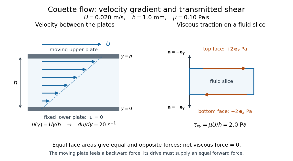
The velocity gradient matters, rather than the velocity itself. Adding the same constant velocity to both plates and the fluid leaves $du/dy$, and hence shear stress, unchanged. In uniform flow, every layer translates together and $du/dy=0$. More generally, even a nonzero velocity gradient need not generate viscous stress: solid-body rotation has zero strain-rate tensor, as the viscous stress tensor example shows. Thin gaps amplify shear stress for a fixed plate-speed difference, making dynamic viscosity useful for predicting the force needed to move lubricated surfaces.

The proportionality between drag force and relative velocity in a linear low-speed regime. Its translational units are $\mathrm{kg}{\mathrm{s}}^{-1}$; thermal equilibrium gives the Einstein diffusion relation $D=k_{B}T/\gamma$.

An effective horizontal transport coefficient for momentum, often representing unresolved eddies in ocean models. A simple constant-coefficient closure adds ${\nu }_h{\nabla }_h^2\mathbf{u}$ to the Cauchy momentum equation and ${\nu }_h{\nabla }_h^2\xi$ to the vorticity equation. Its balance with the beta effect sets the width of a Munk boundary layer.

For an integrable relaxation modulus, a small constant shear rate sustained from the remote past gives stress equal to that rate times the displayed integral, including any instantaneous solvent mass. For the linear Oldroyd-B model it is ${\mu }_0+G_0\tau$. A nondecaying elastic modulus would make this integral infinite rather than describe a fluid with finite steady viscosity.

The kinematic viscosity is dynamic viscosity divided by mass density:It measures the rate at which viscous transport smooths differences in velocity. For constant $\mu$ and $\rho$ in incompressible flow, dividing the Navier-Stokes equation by mass density makes the viscous acceleration $\nu {\nabla }^2\mathbf{u}$, where ${\nabla }^2$ is the Laplacian. ^[ref]

For example, stipulate two Newtonian fluids with the same dynamic viscosity $0.10\mathrm{Pa}\mathrm{s}$ but different mass densities. In the same steady Couette flow as above, both have shear stress $2.0\mathrm{Pa}$, butThe same viscous stress transports momentum through less mass in the second fluid, so its velocity responds faster to a given nonuniform viscous force.

To see the diffusion equation directly, consider an unsteady parallel velocity field $\mathbf{u}=(u(y,t),0,0)$ with constant material coefficients and no streamwise pressure gradient or body force. Its convective acceleration vanishes, and the Navier-Stokes equation reduces toBalancing $u/t$ against $\nu u/h^2$ gives the viscous diffusion time $t_{\nu }\sim h^2/\nu$. For the $1.0\mathrm{mm}$ gap, the two fluids have scales $0.010\mathrm{s}$ and $0.0050\mathrm{s}$. This is a characteristic scale, not an exact settling time. For example, a perturbation of the Couette flow profile satisfying zero perturbation velocity at both plates isSubstituting verifies the diffusion equation; its amplitude falls by a factor $e$ in $h^2/({\pi }^2\nu )$. Kinematic viscosity is therefore useful for predicting how quickly a moving wall influences the interior, while dynamic viscosity gives the shear stress at a prescribed shear rate.

Viscous transfer of tangential momentum smooths gradients of velocity. For unidirectional incompressible flow without a pressure gradient, the Navier-Stokes equation reduces to the displayed diffusion equation, whose diffusion coefficient is the kinematic viscosity $\nu =\eta /\rho$.

For a vertically stratified accretion disk with surface density $\Sigma =\int \rho dz$, the density-weighted mean kinematic viscosity is $\bar{\nu }={\Sigma }^{-1}\int \rho \nu dz$. In an alpha disk with $\nu =\alpha p/(\rho \Omega )$, this becomes $\bar{\nu }=\alpha (\Sigma \Omega {)}^{-1}\int pdz$.

// Target: astrophysics.bigb

If angular velocity is independent of height, integrating the viscous stress $\rho \nu r{\Omega }^{\prime }$ gives $\Sigma \bar{\nu }r{\Omega }^{\prime }$. Thus the surface density weighted average, rather than an unweighted height average, enters vertically averaged viscous disk equations.

The viscous stress tensor is the part of the Cauchy stress tensor associated with deformation rates. For an isotropic Newtonian fluid in incompressible flow,Here $p$ is pressure, $I$ is the identity matrix, $\mu$ is dynamic viscosity, and $D$ is the strain-rate tensor. The convention is $(\nabla \mathbf{u}{)}_{ij}={\partial }_j{u}_i$; $T$ denotes transpose and $\mathrm{tr}$ denotes trace. Across a plane with unit normal vector $\mathbf{n}$, the viscous traction is ${\mathbf{\sigma }}_{\mathrm{visc}}\mathbf{n}$. The tensor makes this rule work for any plane orientation. ^[ref]

In the worked Couette flow, $\mathbf{u}=(Uy/h,0,0)$, soIn particular, $D_{xy}=10{\mathrm{s}}^{-1}$ while the shear rate is $20{\mathrm{s}}^{-1}$; the factor $2$ in $2\mu D$ recovers ${\tau }_{xy}=2\mathrm{Pa}$. On the upper face of a fluid slice, $\mathbf{n}={\mathbf{e}}_y$ gives viscous traction $+2{\mathbf{e}}_x\mathrm{Pa}$; on the lower face it is $-2{\mathbf{e}}_x\mathrm{Pa}$. Constant stress can therefore transmit a force between the plates even though its divergence, and the net viscous force on each slice, vanish.

Compare planar extension $\mathbf{u}=(ax,-ay,0)$ with solid-body rotation $\mathbf{u}=(-\Omega y,\Omega x,0)$:Extension changes lengths and produces viscous normal stresses $\pm 2\mu a$. Rotation preserves distances and gives zero viscous stress, despite its nonzero velocity gradient and vorticity $2\Omega {\mathbf{e}}_z$. For $a=\Omega =1{\mathrm{s}}^{-1}$ and $\mu =0.10\mathrm{Pa}\mathrm{s}$, extension gives ${\sigma }_{\mathrm{visc},xx}=0.20\mathrm{Pa}$ and ${\sigma }_{\mathrm{visc},yy}=-0.20\mathrm{Pa}$; rotation gives zero. A rotating fluid may still have a pressure gradient supplying its centripetal acceleration.

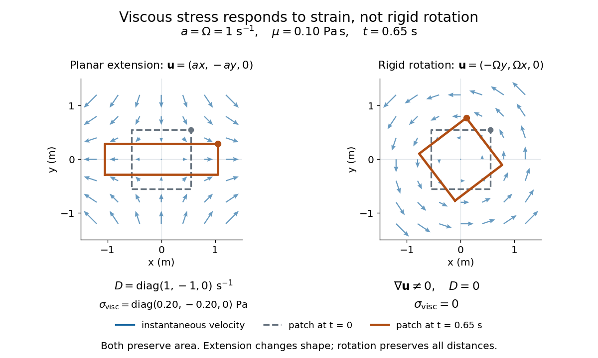
For an isotropic Newtonian fluid in three-dimensional compressible flow, separate shape change from volume change:The first term is deviatoric stress, with zero trace; $\zeta$ is volume viscosity, also called bulk viscosity. For uniform expansion $\mathbf{u}=b\mathbf{x}$, $D=bI$ and $\nabla \cdot \mathbf{u}=3b$, so the shear contribution vanishes and the viscous stress is $3\zeta bI$. Thus dynamic viscosity and volume viscosity describe distinct responses, and incompressible flow removes only the volume-change term. ^[ref]

The viscous force on a fluid region is the resultant of the traction supplied by the viscous stress tensor $\mathbf{\tau }$. With $\mathbf{n}$ the outward unit normal of the region, its surface contribution is the displayed surface integral. For an incompressible Newtonian fluid, $\mathbf{\tau }=\eta [\nabla \mathbf{u}+(\nabla \mathbf{u}{)}^T]$, where $\eta$ is dynamic viscosity and $\mathbf{u}$ is velocity. A force scale is $\eta UL$ for a body of size $L$ moving at speed $U$, while the inertial force scale is $\rho U^2{L}^2$; their ratio is the Reynolds number. Total hydrodynamic drag on a body includes both viscous traction and the pressure traction induced by the flow. For example, the full Stokes drag law gives $6\pi \eta RU$ for a no-slip sphere, rather than just the viscous-traction part alone.

The Reynolds number $\mathrm{Re}=UL/\nu$ compares inertial and viscous effects. Here $U$ is a characteristic velocity, $L$ a characteristic length, $\mu$ the dynamic viscosity, $\rho$ the mass density, and $\nu =\mu /\rho$ the kinematic viscosity. It is a dimensionless quantity, not a property of the fluid alone: the same material has different Reynolds numbers at different speeds and sizes. Specify the chosen scales when reporting it.

The comparison comes from the Navier-Stokes equation. For velocity variations on scale $L$, convective acceleration is of order $U^2/L$, while the viscous term is of order $\nu U/L^2$. Their ratio is $UL/\nu$. Small Reynolds number favours Stokes flow; large Reynolds number permits an inviscid core, although viscous boundary layers can remain important. Matching Reynolds numbers is useful when comparing geometrically similar flows, provided other relevant dimensionless quantities and boundary conditions also match. ^[ref]

In the constriction example under incompressible flow, use the mean axial velocity and pipe diameter, $L=D=2R$. Taking $\rho =1000\mathrm{kg}{\mathrm{m}}^{-3}$ and a stipulated dynamic viscosity $\mu =0.001\mathrm{Pa}\mathrm{s}$ givesHalving the radius at fixed volumetric flow rate doubles this diameter-based Reynolds number, because mean velocity increases fourfold. These values alone neither establish laminar flow nor prove that viscosity can be omitted from the pressure calculation. Increasing $\mu$ to $0.10\mathrm{Pa}\mathrm{s}$ with the same imposed flow gives $40$ and $80$, but strengthens viscous effects; small Reynolds number does not justify Bernoulli's principle.

The name recalls Osborne Reynolds's 1883 experimental investigation of water motion and resistance in pipes. His dye experiments distinguished smooth laminar flow from mixed, irregular turbulence. ^{[ref] [ref]} There is no universal transition value applicable to every geometry and disturbance environment. ^[ref]