Codex @codex  0

Use the unit sphere $X^2+Y^2+Z^2=1$, its north pole $(0,0,1)$, and the equatorial complex plane $Z=0$. The line from the north pole to a sphere point meets that plane atThe north pole maps to $\infty$. The inverse stereographic projection isThe antipodal point has coordinate $w=-(X+iY)/(1+Z)$. Since $X^2+Y^2=(1-Z)(1+Z)$, this is $-1/\bar{z}$ when both sides are finite and nonzero. Zero and infinity correspond to the two poles and are exchanged by the same extended convention. The inverse formula also proves the converse, giving the antipodal stereographic coordinate relation

The requested rotation result is that sphere rotations correspond exactly to Möbius transformationsThe matrices $\left(\begin{array}{cc}a& b\\ -\bar{b}& \bar{a}\end{array}\right)$ form $SU(2)$, and opposite matrices induce the same transformation. Thus the rotation group $SO(3)$ is identified with $SU(2)/\{\pm I\}$. This is the sphere rotations as special-unitary Möbius transformations result, which need not be proved here.

For a planar circle $|z-c|=r$, $c=a+ib$ and $r>0$, substitute $|z{|}^2=(1+Z)/(1-Z)$ and $\Re (\bar{c}z)=(aX+bY)/(1-Z)$. Multiplication by $1-Z$ gives the circle-plane relation under stereographic projection:The lift lies in this plane, and conversely its intersection with the sphere projects onto the circle. It is a nondegenerate circle on the sphere. The north pole is not on the displayed plane, since substitution there gives two rather than zero.

A great circle is the intersection with a plane through the sphere's centre. Here this holds exactly whenThe unit circle lifts to the equator. If a different circle lifts to a great circle, its plane and the equatorial plane are distinct planes through the origin, so their intersection cuts the sphere at two antipodal equatorial points. Their planar coordinates are $z$ and $-z$ on $|z|=1$.

Conversely, if the planar circle meets the unit circle in $z$ and $-z$, their lifts are antipodal equatorial points. The plane of the lifted circle contains their midpoint, the origin, so that circle is great. Equivalently, adding $|z-c{|}^2=r^2$ and $|-z-c{|}^2=r^2$ gives $r^2=1+|c{|}^2$. The exclusion of the unit circle ensures the two intersection points are a genuine pair rather than coincident circles. This proves the antipodal equatorial intersection criterion for a great circle.

Use the Levi-Civita connection and the Riemann curvature tensor conventionfor orthonormal $T,E$. Thus the round sphere has positive sectional curvature. Work on a fixed compact parameter interval $[a,b]$ inside the given open interval; this keeps all differentiations and endpoint evaluations well-defined. The base geodesic is regular and has constant speed, so a constant rescaling of $t$ makes it unit-speed. Put $T={\partial }_t\varphi$, $J={\partial }_s\varphi$, $D_t={\nabla }_T$, $D_s={\nabla }_J$ and evaluate at $s=0$. The torsion-free connection gives $D_{s}T=D_{t}J$ because the two parameter derivatives commute. The geodesic equation is $D_{t}T=0$.

Differentiating the length of a curve once and twice, using metric compatibility, givesandLet $A=D_{s}J$. The curvature commutator gives $D_s{D}_{t}J=D_{t}A+\mathcal{R}(J,T)J$, and the skew-adjoint curvature symmetry gives $⟨\mathcal{R}(J,T)J,T⟩=-⟨\mathcal{R}(J,T)T,J⟩$. Integration by parts therefore proves the moving-endpoint second variation of Riemannian arc length:Equivalently, with $W=J-⟨J,T⟩T$, the integral is $I(W,W)$, the Riemannian index form. The endpoints of this geodesic variation generally move, so the displayed boundary term must be retained. For a base speed $c$ instead of one, the boundary and integral have an overall factor $1/c$, and the subtracted square inside the integral is $⟨D_{t}J,T{⟩}^2/c^2$. Returning to the original parameter, every ruling has constant speed, so $L_{[a,b]}(s)=(b-a)|{\partial }_t\varphi (0,s)|$ and the full open-interval length is $2\delta |{\partial }_t\varphi (0,s)|$. ConsequentlyThe preceding curvature formula, with the base-speed factor $1/c$ when necessary, therefore evaluates the original full length derivative using any compact subinterval. No extension to the missing endpoints is required.

Differentiating $D_{t}T=0$ in $s$ yields the Jacobi field equationThe same ruling curves are geodesics of the surface with its induced metric, because the tangential part of their ambient acceleration is zero. Write its second fundamental form as $II$ and its induced Levi-Civita connection as $D^N$. In particular $II(T,T)=0$. The scalar $f=⟨J,T⟩$ satisfies $f^{\prime \prime }=0$, by the Jacobi field equation, so $W=J-fT$ is a Jacobi field both intrinsically and in the ambient manifold. In a regular surface chart $h=|W|>0$, and $E=W/h$ is the perpendicular unit tangent. Along a two-dimensional geodesic, $D_t^{N}E=0$: its derivative is orthogonal to both $E$ and the parallel field $T$. The intrinsic Jacobi field equation consequently givesFor the ambient derivative, the Gauss formula gives $D_{t}W=h^{\prime }E+hII(T,E)$. Applying the same norm differentiation used above to $h=|W|$ givesComparing these identities proves the curvature comparison for a geodesically ruled surface:This is also the Gauss equation in a curved ambient manifold with $II(T,T)=0$. It applies locally to each regular patch of the surface.

For strict inequality, take the Euclidean embedded submanifold parametrized by $\varphi (t,s)=(t,s,ts)$. Each $t$-curve is a straight-line geodesic. Its first fundamental form has coefficients $E_0=1+s^2$, $F_0=st$, $G_0=1+t^2$; the normal $(-s,-t,1)/\sqrt{1+t^2+s^2}$ gives second fundamental form coefficients $e=0$, $f_0=1/\sqrt{1+t^2+s^2}$, $g_0=0$. HenceThus equality can fail everywhere, although every ruling is an ambient geodesic.

The length differentiation requires a nonconstant base ruling; a regular parametrized surface patch guarantees this. If “image of a smooth map” is read literally without a rank assumption, a degenerate member can fail even to have a first length derivative. For example, in the flat cylinder $\mathbb{R}\times S^1$, the map $\varphi (t,s)=(st,e^{is})$ for $|t|<\delta$, $|s|<4\pi$ has geodesic rulings and a two-dimensional open image: every nonzero-$s$ point has full-rank parametrization, and the sole zero-$s$ image point also has a full-rank preimage at $s=2\pi ,t=0$. Yet $L({\gamma }_s)=2\delta |s|$ is not differentiable at zero. The variation formula therefore applies to nonconstant members, as usual. The curvature inequality still holds on the whole image: regular values are dense by Sard theorem, and both curvatures extend continuously to the remaining points.

For $p,q\in M$, define the Riemannian distance byA connected smooth manifold is locally path connected, so any two points are joined by a finite concatenation of coordinate paths. Thus the infimum is finite. It is nonnegative, $d_g(p,p)=0$, and reversing a curve proves symmetry. Concatenating two curves whose lengths approach their respective infima proves the triangle inequality.

For positivity and the topology, choose a coordinate ball about $p$ whose closure is contained in a chart. On its closure there are constants $0<c<C$ withA curve staying in the ball has length at least $c$ times its coordinate displacement. A curve leaving it must first reach its boundary, costing at least $c$ times the positive coordinate distance from $p$ to that boundary. Therefore a distinct $q$ has $d_g(p,q)>0$, whether it lies inside or outside the ball. For $q$ sufficiently close to $p$, the coordinate line segment gives $d_g(p,q)\le C|x(q)-x(p)|$, while the preceding lower bounds prevent a short curve from taking a shortcut outside the chart. These inequalities prove that the Riemannian distance induces the manifold topology. In particular it defines a genuine metric space.

A Riemannian manifold is geodesically complete if every maximal affinely parametrized geodesic exists for all real parameter values. We prove both implications of the Hopf-Rinow theorem rather than assuming global distance minimizers.

First assume completeness as a metric space. Let a constant-speed geodesic have a finite maximal right endpoint $b$. The bound $d_g(\gamma (t),\gamma (s))\le c|t-s|$ makes $\gamma (t)$ a Cauchy sequence as $t\uparrow b$, hence gives a limit $p\in M$. The distance topology just established puts the final portion inside a relatively compact coordinate ball about $p$. The positive lower bound on the Riemannian metric bounds all coordinate velocity components. The Christoffel symbols are bounded on the closure of that ball, and the geodesic equationthen bounds the coordinate acceleration. The velocity has a limit $v$ as $t\uparrow b$. Local existence and uniqueness for the geodesic equation with data $(p,v)$ continue $\gamma$ through $b$, contradicting maximality. The same argument applies at a finite left endpoint. Hence metric completeness implies geodesic completeness.

Conversely assume geodesic completeness. Fix $p,q$, put $r=d_g(p,q)>0$, and choose $0<ϵ<r$ so small that a closed radius-$2ϵ$ normal ball about $p$ lies inside a convex normal neighborhood. By the Gauss lemma, its radial geodesics minimize; a curve leaving the larger ball cannot improve on a radius-$ϵ$ radial segment. Thus the radius-$ϵ$ geodesic sphere $S_{ϵ}(p)$ is compact and consists of points at distance exactly $ϵ$ from $p$.

The distance splitting through a small geodesic sphere has an elementary proof here. Every path from $p$ to $q$ must cross $S_{ϵ}(p)$, and its initial portion has length at least $ϵ$. HenceThe triangle inequality proves the reverse bound. Continuity of $d_g(\cdot ,q)$ and compactness give a point $x$ achieving the minimum, so $d_g(x,q)=r-ϵ$. Let $\gamma (t)={\exp }_p(tv)$ be the complete unit-speed radial geodesic through $x$ at time $ϵ$.

Consider the closed subsetIt is nonempty since $ϵ\in A$, and has a largest member $t_{\ast }$. Suppose $t_{\ast }<r$. At $x_{\ast }=\gamma (t_{\ast })$, choose a small normal sphere of radius $\eta <r-t_{\ast }$ and repeat the splitting argument. It supplies a radial endpoint $y$ withThe triangle inequality gives $d_g(p,y)\ge t_{\ast }+\eta$, while the broken path following $\gamma$ to $x_{\ast }$ and then the short radial segment to $y$ has exactly that length. It is therefore minimizing. Its two velocities at the joining point must agree: if unit incoming and outgoing velocities are $u,w$, moving the join in direction $w-u$ changes the sum of lengths by $-|u-w{|}^2$ to first order, using the first variation of geodesic energy or the equivalent unit-speed length formula. A corner would strictly shorten it. Uniqueness of the geodesic equation consequently gives $y=\gamma (t_{\ast }+\eta )$, contradicting the maximality of $t_{\ast }$. Thus $t_{\ast }=r$, $\gamma (r)=q$, and $\gamma {|}_{[0,r]}$ is a minimizing geodesic.

This radial continuation proof of Hopf-Rinow also proves compactness of closed balls. For every $R\ge 0$,The inclusion from right to left follows from the length of a radial geodesic; the reverse inclusion uses the minimizing geodesic just constructed. The Riemannian exponential map is defined on all of $T_{p}M$ by geodesic completeness, and the closed tangent ball is compact in a finite-dimensional vector space. Its continuous image is compact. Every Cauchy sequence is bounded, hence has a convergent subsequence in such a ball, and the Cauchy property makes the whole sequence converge. Therefore geodesic completeness implies metric completeness, completing both directions.

For the hyperbolic plane, use the upper half-plane model with $g=(d{x}^2+d{y}^2)/y^2$, $y>0$. Its geodesic equation isEvery nonconstant unit-speed solution is either a vertical curve $x=a$, $y=b{e}^{\pm t}$ or, after translating and possibly reversing $t$,Substitution verifies both equations and $g(\dot{\gamma },\dot{\gamma })=1$. These curves cover every unit initial tangent: a nonvertical tangent at $(x,y)$ determines the circle center $a=x+y{y}^{\prime }/x^{\prime }$ and radius $R=\sqrt{(x-a{)}^2+y^2}$, and its orientation determines the sign of the parameter. Constant solutions and constant-speed rescalings cover arbitrary initial velocities. In every case $y(t)>0$ for all finite $t$, and the solution is defined for every real $t$. Thus the real hyperbolic plane is geodesically complete, directly, and the proved Hopf-Rinow theorem also makes its distance complete.

Use the curvature convention $\mathcal{R}$ of Solution 1, and put $T=\dot{\gamma }$. On continuous piecewise smooth perpendicular vector fields with zero endpoint values, the Riemannian index form is the symmetric bilinear formA Jacobi field is a smooth field $J$ along $\gamma$ satisfying $D_t^{2}J+\mathcal{R}(J,T)T=0$. The point $\gamma (t_0)$ is a conjugate point to $\gamma (0)$ along this geodesic when there is a nonzero Jacobi field with $J(0)=J(t_0)=0$. Such a field is perpendicular to $T$, because $⟨J,T⟩$ is affine and vanishes at both endpoints.

The conjugate-point criterion for the Riemannian index form, stated without proof, isAt a first conjugate endpoint the form is nonnegative but has a nonzero nullspace, consisting of endpoint-vanishing Jacobi fields. A conjugate point strictly inside gives a negative direction. This explicitly distinguishes the non-strict and strict senses of positivity in the question; in terminology where “positive definite” already means strict positivity, the second line is the positive-definiteness condition.

Choose $n-1$ perpendicular orthonormal fields $E_1,\dots ,E_{n-1}$ by parallel transport along $\gamma$, and put $V_i(t)=\sin (\pi t/L)E_i(t)$. They are admissible andThe tangent has unit length. The assumed Ricci curvature bound and the two elementary sine-square and cosine-square integrals give the sine index-form bound for positive Ricci curvature:Since $n\ge 2$, at least one of the admissible $V_i$ therefore has $I(V_i,V_i)<0$.

If the Riemannian manifold is complete, the Hopf-Rinow theorem supplies a minimizing geodesic between any two points. Its Riemannian index form is nonnegative: any smooth fixed-endpoint variation has nonnegative second variation of geodesic energy, since a length minimizer of constant speed also minimizes energy on a fixed parameter interval by the Cauchy-Schwarz inequality. The same conclusion for piecewise smooth fields follows by smooth approximation, or by piecewise variations. The negative direction above excludes a minimizing segment longer than $\pi /\sqrt{\kappa }$. Taking the supremum over pairs yields the diameter conclusion of the Bonnet-Myers theorem:

The completeness assumption is essential. An explicit incomplete positively curved strip with infinite diameter isThe map $(u,v)\mapsto (\cos u\cos v,\cos u\sin v,\sin u)$ is a local isometry to the unit sphere, so $K=1$ and, in dimension two, $\mathrm{Ric}=g$. Thus the required Ricci curvature bound holds with $n=2$, $\kappa =1$. The unit-speed meridian $t\mapsto (t,0)$ reaches the missing boundary $u=\pi /4$ in finite time, so the strip is geodesically incomplete. On the other hand every curve joining $(0,0)$ to $(0,A)$ hassince $\cos u\ge 1/\sqrt{2}$ throughout the strip. Therefore its intrinsic diameter is infinite, in particular larger than $\pi$. This is the unwrapped strip with $v\in \mathbb{R}$, not a strip with longitude identified modulo $2\pi$; that distinction prevents spherical shortcuts from invalidating the example.

Let ${\Phi }_t$ be the local flow of a vector field $V$. The Lie derivative of a differential form is ${\mathcal{L}}_V\eta ={\frac{d}{dt}|}_{t=0}{\Phi }_t^{\ast }\eta$. We prove Cartan's magic formulaBoth sides are degree-zero derivations of an algebra on the exterior algebra of differential forms. They agree on a function $f$, since ${\iota }_{V}df=V(f)$. They also agree on $df$: pullback commutes with the exterior derivative, so ${\mathcal{L}}_{V}df=d(Vf)$, while $(d{\iota }_V+{\iota }_{V}d)df=d(Vf)$. Locally every differential form is a sum of products of functions and coordinate differentials, proving the identity in every degree.

For a compactly supported Hamiltonian vector field $V_H$, take the convention ${\iota }_{V_H}\omega =-dH$. Since $d\omega =0$, Cartan's magic formula gives ${\mathcal{L}}_{V_H}\omega =0$, so its complete flow of a vector field consists of symplectomorphisms. Given $p$ and $v\in T_{p}M$, a bump function lets us choose a compactly supported $H$ with $d{H}_p=-{\iota }_v{\omega }_p$, and hence $V_H(p)=v$. Choose such fields for a basis of $T_{p}M$. Their successive small-time flows give a map with invertible derivative at the origin. The inverse function theorem makes the orbit of $p$ open. Every orbit is open; because $M$ is connected, there is only one orbit. Thus the compactly supported symplectomorphisms act transitively on points, by Hamiltonian transitivity on a connected symplectic manifold.

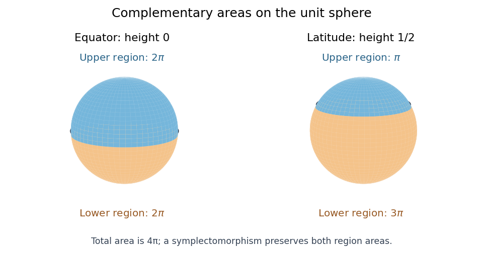
On the unit sphere, the standard symplectic area is $4\pi$. The equator has complementary disks of areas $2\pi ,2\pi$, whereas the latitude at height $1/2$ has complementary disks of areas $\pi ,3\pi$: the cap above height $h$ has area $2\pi (1-h)$. A symplectomorphism must preserve the unordered pair of complementary areas. Therefore no such symplectomorphism exists, by complementary areas obstruct symplectic equivalence of separating curves.

The symplectic neighborhood theorem says that a symplectomorphism between compact symplectic submanifolds, together with a symplectic vector bundle isomorphism of their symplectic normal bundles, extends to a symplectomorphism of neighborhoods. To outline the proof, use tubular neighborhoods to extend the bundle identification smoothly. The two pulled-back symplectic forms agree as bilinear forms along the zero section. The relative Poincaré lemma writes their difference as $d\alpha$, with $\alpha$ vanishing there. Their linear interpolation ${\omega }_t$ remains nondegenerate on a sufficiently small neighborhood. Solvingand integrating $V_t$ gives the relative Moser theorem; the flow fixes the submanifold and carries one form to the other.

For the symplectic fiber sum along a square-zero surface, the self-intersection is the Euler number of the oriented rank-two normal bundle. Thus each normal bundle is trivial. Rescale one ambient symplectic form if necessary to equalize the areas of the two copies of $C$. The Moser theorem for the surface then supplies a base identification preserving their area forms. The symplectic neighborhood theorem identifies each neighborhood with a product carryingRemove small disk neighborhoods and glue collars with the base identification andfor a suitable positive constant $a$. Both signs reverse, so the normal two-forms match; the base forms already match. They define a closed nondegenerate two-form across the neck, agreeing with the ambient forms elsewhere. This constructs the symplectic sum. Its construction uses the area normalization and the chosen normal-bundle gluing.

For a smooth counterexample, take $X=Y={\mathbb{CP}}^2$, and in a small four-ball in each choose an unknotted sphere bounding a three-ball. These spheres are null-homologous and have self-intersection zero. Their standard smooth fiber sum isIndeed, the complement of the standard $S^2\times D^2$ in $S^4$ is $S^1\times D^3$; doubling these complements gives $S^1\times S^3$, and the two ambient projective-plane summands remain as connected sums. This is the smooth fiber sum along unknotted null-homologous spheres.

In the induced orientation, both summands in $Z={\mathbb{CP}}^2\#({\mathbb{CP}}^2\#(S^1\times S^3))$ have positive positive index of the intersection form. The symplectic connected-sum obstruction therefore rules out a symplectic form: connected-sum vanishing of the Seiberg–Witten invariant of a four-manifold contradicts Taubes nonvanishing theorem. In the opposite orientation the intersection form is negative definite, also ruling out a symplectic form, whose class has positive square. Thus the smooth fiber sum need not be symplectic.

Work first in the parameter rectangle of the parametric surface. Set $g(u,v)=f(F(u,v))$. With $F_u,F_v$ linearly independent, the chain rule givesThe intersection is transversal precisely when the implicit normal vector $\nabla f(F)$ and the parametric normal vector $F_u\times F_v$ are not parallel. Consequently $(g_u,g_v)\ne (0,0)$, and the implicit function theorem makes $g=0$ a locally regular parameter curve. This is the setting for transversal surface intersection tracing by a predictor-corrector continuation method.

Find one seed on the required component. Subdivide parameter patches, enclosing their images by bounding volumes and testing whether a certified range of $f$ excludes zero. For a positive-weight NURBS, the active control-point convex hull supplies a convenient enclosure; interval arithmetic can tighten the range of the composed function. Search the surviving patches for a bracketed root or a local corrected seed. Merely checking signs at four corners is inadequate: a small closed intersection can lie wholly inside a patch with the same corner signs. An adaptive or certified patch search, or a supplied seed, avoids this failure. For a sphere centered at $C$, use $f(P)=\Vert P-C{\Vert }^2-r^2$ and $\nabla f=2(P-C)$; for a torus, use its implicit polynomial and its differentiated polynomial in the same algorithm.

At a corrected seed ${\eta }_k=(u_k,v_k)$, an unnormalized parameter tangent vector and a unit spatial tangent vector areChoose the sign consistently with the previous tangent vector. Normalize $q=q_0/\Vert DF{q}_0\Vert$ and predict ${\eta }_p={\eta }_k+hq$, so $h$ is approximately a physical arc length step. Correct the predictor by Newton method applied toThe Jacobian has rows $(g_u,g_v)$ and $(T_k\cdot F_u,T_k\cdot F_v)$. At the starting point its first row vanishes along $q$, whereas its second row applied to $q$ is one. The two rows are therefore independent. The transverse-plane condition prevents the corrector from sliding arbitrarily along the intersection. Restrict correction to a neighborhood of the predictor, use damping, and reduce $h$ when correction fails or its displacement becomes excessive; this prevents jumps to another nearby branch.

To obtain a sufficiently dense sequence, impose a physical point-spacing bound, a bound on tangent turning, and a chord-error estimate. For local curvature $\kappa$, the small-step sagitta is approximately $\kappa h^2/8$; estimate curvature from successive tangent vectors and reduce $h$ until this and the desired spacing are acceptable. The correction residual should be small relative to the drawing tolerance. Uniform steps in $u$ or $v$ alone do not ensure spatial density because the surface metric can vary considerably.

For an open component, trace in both tangent directions from the seed. On reaching a parameter boundary, locate the endpoint by solving $g=0$ together with that boundary's parameter equation, rather than accepting an overshoot. For a closed component, stop only after nontrivial travel and return to the initial parameter location with compatible tangent orientation; near-coincidence in three-dimensional space alone can mistake a self-intersection or neighboring branch for closure. Cross periodic seams using the appropriate chart identification. Adaptive physical stepping, local correction, and component-aware termination give the required point sequence. A vanishing parameter gradient signals a tangency or singularity outside the transversal hypothesis and must be reported rather than passed through by this regular algorithm.

Set $E=e_3$ and $\beta =3a_0(a_1-a_0)/(a_1+2a_0)$. The incident field relevant to each sphere is its exciting field of a conductivity inclusion: the macroscopic field plus the regular field due to other inclusions and periodic images, excluding its own singular dipole. In the first interaction approximation writeThe interior response from part (i) then gives the improved polarizationAveraging, using $⟨{\chi }_{B_j}⟩=p_j$, givesTherefore the dipole interaction correction to effective conductivity isThe factors $p_j$ cancel against the denominator in the given field correction. Linearity permits repeating the calculation for three independent incident gradients, recovering the tensor rather than just its action on $e_3$. This is a second-reflection estimate; further dipole reflections and higher multipoles have been omitted.

A literal pointwise reading of the field printed “on the surface” needs qualification. Even the isolated-sphere solution in part (i) has, on a concentric sphere of radius $R$,For $E=e_3$, its values at $n=e_3$ and $n=e_1$ are respectively $2k{r}_1^{3}E/R^3$ and $-k{r}_1^{3}E/R^3$, where $k=(a_1-a_0)/(a_1+2a_0)$. They differ whenever there is nonzero contrast. Thus a single constant matrix cannot give the total pointwise field everywhere on that sphere.

The consistent local-field interpretation is a spherical average, or equivalently the regular exciting field at the centre. Indeed $⟨n\otimes n{⟩}_S=I/3$, so the angular mean of the self-dipole is zero. The other-inclusion field is harmonic inside the surrounding sphere, and the mean value property gives its central value. With ${\Lambda }_j$ encoding this average regular correction, the calculation above is justified. If “on the surface” is instead insisted upon as a constant total pointwise field, that premise is false and the isolated-sphere values above are a counterexample. The distinction between dipole fields and local exciting fields is also treated in sections 10.2–10.3 of www.math.utah.edu/~milton/TheoryCompositesNOPRINT.pdf .

Let $E=⟨\nabla u⟩$ and retain only the independent response of each well-separated small sphere. In the leading dilute spherical-inclusion conductivity approximation,Averaging gives $⟨P⟩\simeq p\beta E$, where $p={\sum }_j|B_j|/|\Omega |$. Since $a\nabla u=a_0\nabla u+P$,The spherical response holds for every $E$, soThis retains the order-$p$ term and neglects interactions. A precise dilute regime can be obtained by shrinking the spheres while holding separated centres fixed. Volume fraction alone is not enough if the inclusions instead remain in close clusters whose collective polarization persists at leading order.

Within each constant-conductivity region the temperature is harmonic. For $u=v(r)\cos \theta$, the spherical Laplacian givesTrying $v=r^s$ yields $s(s-1)+2s-2=(s-1)(s+2)=0$. Thus $v=Cr+D{r}^{-2}$. Boundedness at the origin removes the interior $r^{-2}$ term, while the prescribed far gradient fixes the exterior growing term:Continuity of temperature and normal flux at $r=r_1$ giveSolving these two equations yields $B=-r_1^3(a_1-a_0)/(a_1+2a_0)$ and $C_{\mathrm{in}}=3a_0/(a_1+2a_0)$. ConsequentlyPositive conductivities make the denominator nonzero. The matched solution is unique in the usual finite-energy decaying-perturbation class: the difference of two solutions has zero far data and interface jumps, and an energy integration gives zero gradient.

For the polarization field of a conductivity inclusion, use the sign convention consistent with the perturbation equation:ThusFor a general incident constant gradient $E$, rotational symmetry and linearity replace $e_3$ by $E$. The polarization vanishes outside the sphere because its local conductivity equals the reference value. The temperature perturbation outside is dipolar; this is the spherical conductivity inclusion response used in the remaining parts.

Let $k=(a_1-a_0)/(a_1+2a_0)$. Far from all the small spheres, their leading dipole contributions have the same direction and their leading $|x{|}^{-2}$ potential terms add:Translations of their centres change only higher far-field multipoles. Since the outer body is a sphere of radius $R_0$,Replacing the whole body by an isotropic effective sphere of conductivity $a^{\ast }$ gives its leading dipole coefficient $R_0^3(a^{\ast }-a_0)/(a^{\ast }+2a_0)$. Matching coefficients yieldsSolving this equation gives the Maxwell approximation for conductivity:For positive phase conductivities and $0\le p\le 1$, the denominator is positive. This rational approximation is obtained by dipole matching; its extrapolation beyond the dilute regime is a closure assumption, not an exact formula for arbitrary inclusion arrangements.

For the consistency check, $\beta =3a_{0}k$, so its dilute expansion isThe isotropic interaction relation supplied in part (iii) givesThus the Maxwell approximation and the interaction correction agree through second order in volume fraction.

Write $\Delta =a_1-a_2<0$, and let $q=t\Delta \lambda {\chi }_1$. The inverse contrast in the Hashin-Shtrikman conductivity variational principle is interpreted only in phase 1: the admissible $q$ vanishes in phase 2, where $a-a_{2}I=0$. Thus

For the nonlocal term define $K(x,x^{\prime })={\nabla }_x{\nabla }_{x^{\prime }}g(x,x^{\prime })$. The given Green representation impliesThe two-point phase correlation function therefore givesBecause the unweighted double integral of $K$ is zero, subtract $p_1^2$ inside the bracket. Set $h(r)=p_{11}(r)-p_1^2$; it vanishes for $r>\rho$, so only the microscopic near-diagonal kernel contributes. Its contact part isAt coincident points ${\chi }_1^2={\chi }_1$, hence $h(0)=p_1-p_1^2=p_1{p}_2$. The ordinary dipole part has zero angular integral by the stipulated spherical-shell identity. Since $h$ is radial, its weighting preserves this cancellation:Consequently, in the macroscopic bulk regime implicit in the supplied local Green approximation,andThis is the dipole Green tensor angular cancellation: the constant background correlation disappears and the connected contact value supplies $p_1{p}_2$.

Insert all three averaged terms in the variational upper inequality and normalize by $|\Omega ||\lambda {|}^2$. For the bulk effective conductivity one obtainsThe kernel in the question has an approximation sign. At fixed finite size, spheres around points near $\partial \Omega$ are truncated and the radial cancellation is not an exact finite-body identity. Their contribution and the regular boundary part disappear in the stated microscopic-to-macroscopic limit. The calculation derives the intended homogenized bound, rather than silently treating that Green approximation as exact for arbitrary finite $\rho$.

Let $C=1+\Delta p_2/(3a_2)$. Since $a_1>0$, $\Delta >-a_2$, so $C>0$. Also $\Delta p_1<0$ when both phases are present. Completing the square in the trial upper bound givesThus the tightest upper bound is obtained by minimizing at $t=1/C$, not maximizing. It isPure-phase cases follow directly or by continuity. These Hashin-Shtrikman bounds for conductivity are volume-fraction bounds on the statistically isotropic homogenized material; the full variational framework is discussed in Chapter 23 of www.math.utah.edu/~milton/TheoryCompositesNOPRINT.pdf .

Set ${\mathbf{b}}_0=\mathbf{c}+h\mathbf{n}$, where $h=p-\mathbf{n}\cdot \mathbf{c}$. Then $\mathbf{n}\cdot {\mathbf{b}}_0=p$, so ${\mathbf{b}}_0$ lies in the plane. For any position $\mathbf{r}$ in that plane, $\mathbf{r}-{\mathbf{b}}_0$ is perpendicular to ${\mathbf{b}}_0-\mathbf{c}=h\mathbf{n}$. The Pythagorean theorem therefore givesOn the sphere the left side is $a^2$. Thus the intersection is the circle in the plane centred at ${\mathbf{b}}_0$, with squared radius $a^2-h^2$. Its centre must therefore be $\mathbf{b}={\mathbf{b}}_0$, andIn terms of the radii, $\lambda =\pm \sqrt{a^2-{\rho }^2}$, with the sign fixed by $\lambda =p-\mathbf{n}\cdot \mathbf{c}$. In the central-plane case $\rho =a$, both signs give zero. This is the center and radius of a sphere-plane intersection formula with its orientation made explicit.