Write for enclosed mass. The stellar hydrostatic equation is . If radiation pressure dominates, compare it directly with the radiative diffusion result for :
This is the limiting Eddington luminosity scaling, assuming fixed composition and electron-scattering opacity.
If gas pressure dominates, use stellar homology: characteristic density and pressure . The ideal gas law then gives
Estimating in radiative diffusion gives
Thus at fixed and constant electron-scattering opacity, . These are stellar homology estimates for radiative stars, not exact relations valid for arbitrary composition and internal transport.
The same gas-pressure stellar homology estimates give and . With Kramers' opacity law , radiative diffusion gives
Consequently the claimed exponent five additionally requires the approximate low-mass main-sequence mass-radius relation and fixed composition:
The supplied opacity and pressure assumptions alone do not establish that mass-radius relation. For example, a homologous fixed-radius family obeys those scaling assumptions but gives , not . More generally gives . Very low-mass stars can be convective, where this radiative model ceases to apply.
To distinguish the companion, measure the host's radial velocity reflex motion to infer a mass; a low-mass star generally produces a much larger signal than a planet. Also test for a detectable secondary eclipse, colour-dependent dilution, doubled spectral lines and out-of-eclipse ellipsoidal variation. High angular-resolution imaging and shifts of the image centroid can identify a blended background eclipsing binary. A Jupiter-sized radius alone is not decisive because low-mass stars and brown dwarfs can have comparable radii. The three labelled effects on the transit are treated individually below.
If radiation dominates the central pressure, equate to . This gives
At roughly fixed burning temperature, the corresponding mass-radius scaling is , rather than the gas-pressure estimate . Radiation pressure alone does not determine a unique radius at a specified mass: a thermal or nuclear-burning condition is still needed to specify . The relation is a homology estimate, not a universal exact law for all massive stars.
The numbered features in the original colour-magnitude diagram have the following interpretation.
Continuous star formation explains the coexistence of newly formed massive main-sequence stars with evolved low-mass remnants; interpreting a single sharp turnoff as the age of a coeval cluster would be inappropriate here.
Multiply hydrostatic equilibrium by and integrate from centre to surface. Integration by parts, neglecting external surface pressure, gives
For an ideal gas with a constant adiabatic index, . Consequently
A fully ionized, nonrelativistic monatomic gas has , provided gas rather than radiation or degeneracy dominates the thermal equation of state. It then obeys and .
Added nuclear heat initially raises pressure and causes expansion. The expansion makes gravitational energy less negative and can lower the temperature of the self-gravitating gas, reducing the temperature-sensitive fusion rate. Conversely, a small contraction can raise the core temperature and increase burning. This negative feedback explains stable main-sequence burning in an ordinary nondegenerate stellar core; a degenerate core need not respond the same way.
Before hydrogen ignition, a cloud loses energy by radiation and contracts. Its gravitational energy decreases; for the ideal-gas virial relation, roughly half the released binding energy heats the gas and half is radiated. Heating continues until nuclear reactions can balance the luminosity, explaining the Kelvin-Helmholtz phase of pre-main-sequence evolution.
The effective adiabatic response varies with ionization, molecular dissociation, radiation pressure and degeneracy. Partial ionization can absorb compression energy and lower the local first adiabatic exponent below , encouraging compressibility, convection and pulsational instability. A local outer layer with does not by itself prove global collapse: ordinary stars have ionization layers of that kind. The dynamical stability criterion concerns a suitable pressure-weighted global response and its coupling to the eigenmode; an extended star with an effectively global exponent below can be dynamically unstable.
The radiation pressure at a photospheric temperature near K is only about Pa. For an illustrative photospheric gas density and mean molecular weight near , the ideal gas pressure is about Pa. Thus gas pressure dominates those outer layers by many orders of magnitude. Both the temperature and density are needed: low temperature alone is not a complete comparison.
For homologous stars, hydrostatic and ideal-gas estimates give and . Therefore
with a structural coefficient independent of mass only under the homology assumption. As mass rises, radiation becomes increasingly important. A rough solar interior normalization of - suggests equality after a mass increase by tens, while realistic radiation-dominated structure and composition shift the scale; stars of order are a useful estimate for strong radiation support. The very small photospheric ratio must not be used as a universal normalization for their whole interiors.
Radiation also transfers outward momentum. Comparing radiative acceleration with gravity gives the Eddington luminosity
Near this scale, radiatively driven winds and envelope instabilities can remove matter or impede further accretion. Opacity, composition, rotation, mass loss and formation history affect the limiting stellar mass. The Eddington condition is a luminosity-to-mass constraint, not a unique composition-independent maximum stellar mass.
Use characteristic stellar values in the supplied radiative temperature gradient: . Hence . With Kramers opacity, ,
Hydrostatic support by an ideal gas gives , or . Substitution then yields
The result assumes homologous density and temperature profiles, comparable structural constants, gas-pressure support and radiative transport throughout. It is not simultaneously an electron-scattering-opacity result; replacing Kramers opacity changes the exponents. Convection, degenerate cores or a different opacity regime limit quantitative application to real evolved helium stars.
Fully ionized helium supplies three particles per four hydrogen masses, so . The same small , but negligible hydrogen fraction, gives , half the hydrogen-star coefficient. The relative luminosity is
Consequently
The very strong molecular-weight dependence outweighs the reduction in mass. Treating the two opacities as identical would miss a factor two, and using neutral-gas molecular weights would be inconsistent with the stated hot ionized stars.
For fully ionized hydrogen with a small metal fraction, there is approximately one proton and one electron per hydrogen mass, so . The Kramers coefficient is proportional to . Denote this star's luminosity by ; the supplied proportionality law alone does not fix its absolute normalization.
Relative to the helium-dominated comparison star, the calculation in part ii gives
If one uses a roughly solar luminosity as an illustrative calibration for this roughly solar-mass, solar-central-temperature reference, the helium star would be of order a hundred solar luminosities. That calibration is only approximate because a mostly hydrogen composition with is not the actual solar composition.
Core-helium-burning stars populate the horizontal branch and red clump; hot subdwarf B stars provide examples with a helium-burning core of roughly half a solar mass and a very small remaining hydrogen envelope. Their high luminosity relative to mass, hot spectra and locations away from an ordinary hydrogen-burning main sequence are observational evidence for such evolved configurations.
A plausible history starts with a hydrogen-burning star. After central hydrogen exhaustion, hydrogen-shell burning builds a compact helium core and the envelope expands on the red giant branch. Sufficient core temperature ignites helium, often by a helium flash for a low-mass degenerate core. Strong mass loss or binary interaction can strip most of the hydrogen envelope, exposing a hot helium-burning remnant; retaining a substantial envelope instead gives an ordinary horizontal-branch or red-clump star.
The simple radiative Kramers scaling estimates a luminosity contrast but does not uniquely identify one evolutionary state or predict a real subdwarf luminosity precisely. A similarly low-mass helium white dwarf would be a cooling, degenerate object rather than the sustained high-temperature helium-burning configuration assumed here.
The sequence primarily orders effective temperature rather than chemical composition. Hot O spectra show strong ionized-helium features and highly ionized metals, with relatively weak neutral-hydrogen lines. B stars show neutral helium and increasingly prominent hydrogen. A stars have the strongest Balmer absorption. Through F and G, lower-ionization metal lines and calcium features become prominent. K stars have strong low-ionization metal absorption and cool-star features; M stars develop strong molecular bands such as TiO, while Balmer absorption is weak.
Line opacity depends on how many atoms occupy both the relevant ionization stage and the particular lower level. Boltzmann excitation controls the latter and Saha ionization the former, so equal elemental abundances need not give equal line strengths. Electron pressure, surface gravity, broadening and atmospheric temperature gradients also affect the spectrum.
For Balmer absorption the lower state is , eV above the hydrogen ground state. In cool atmospheres its population is exponentially small. At higher temperatures it rises, but at still higher temperature ionization removes neutral hydrogen. The competition gives the maximum in A-type stars, with effective temperatures around - K. This is an excitation-and-ionization effect, not evidence that A stars have the largest hydrogen abundance.
A K-star-like integrated spectrum indicates that old or intermediate-age cool stars, often luminous red giants, dominate the observed optical/near-infrared light. It suggests little ongoing formation of very luminous hot O and B stars. It does not imply that every star is K type: faint low-mass dwarfs and remnants can contribute substantial mass while contributing little light.
Using the reference wavelength printed in the problem,
The low-redshift Hubble estimate is
Peculiar velocities and the distinction between luminosity and angular-diameter distance introduce percent-level or larger corrections to this simple estimate. The numerical result intentionally uses the supplied calcium reference rather than replacing it with a different tabulated line wavelength.
The integrated spectrum combines stars moving toward and away from us within the galaxy, broadening their absorption by Doppler shifts. Assuming instrumental and individual-stellar widths have been removed or are negligible, the line-of-sight velocity dispersion is
The angular half-light radius at the low-redshift distance is kpc. For a pressure-supported, approximately isotropic equilibrium spheroid with a standard structural virial coefficient of order five, use
The coefficient represents assumed density profile, aperture and orbital structure; a different reasonable mass estimator changes the result by an order-unity factor. Treating as a luminosity distance and using would reduce the radius and mass by about four percent here.
The distance modulus is about . The magnitude within therefore corresponds to and
Doubling the half-light luminosity gives
This ratio is compatible with an old stellar population plus possible dark matter. It is larger than a solar-like mass-to-light ratio, but does not by itself isolate a unique dark-matter fraction: stellar age, initial mass function, anisotropy and the virial coefficient are not specified. Counting the quoted half-light magnitude as the total would incorrectly double the inferred ratio.
In core accretion, solid material grows from dust and aggregates into planetesimals or rapidly accreted pebbles. A sufficiently large core binds an atmosphere; beyond the snow line, additional condensed volatiles aid solid growth. Cooling allows the envelope to contract and acquire more gas. Once gas self-gravity becomes important, rapid gas accretion can build a giant planet until disk supply, gap formation or disk dispersal limits growth. Migration and interactions with other bodies can alter its final orbit.
Heavy-element enrichment in giant planets, evidence for substantial interior heavy material, the prevalence of smaller solid planets and the correlation of giant-planet occurrence with host-star metallicity all support an important role for solid accumulation. They do not uniquely establish one growth pathway. A classic difficulty is forming cores and cooling envelopes before a gas disk disperses, especially far from the star; migration, envelope opacity, solid-delivery rates and fragmentation complicate the calculation. Pebble-assisted growth can change the timescale, and disk gravitational instability remains a distinct possible route in some environments.
Planetary luminosity is the total emitted power. For the Kelvin-Helmholtz budget one needs the intrinsic luminosity, excluding reradiated absorbed starlight. With orbital distance , Bond albedo , solar luminosity and present-like radius ,
The given ratio of emitted to absorbed power is , so . Using the supplied radius, AU and a solar luminosity around W gives
consistent with the quoted W. Taking as intrinsic power would incorrectly include reradiated sunlight.
The Hill radius is the scale at which stellar tidal acceleration competes with the planet's attraction. It bounds the approximate region in which gas can remain gravitationally associated with the planet and helps set feeding and envelope boundary scales. With a Jupiter mass,
Using this as the stipulated extended proto-planet radius and the present-like intrinsic luminosity gives
Using the compact present radius instead would give an even longer value, of order years at that same luminosity. Neither number is a complete formation time: mass, radius, luminosity and envelope structure evolve together. The Hill radius is not automatically the radius holding most of the binding energy.
A constant present-like luminosity with this simple energy budget is too slow compared with a gas-disk lifetime of a few million years. At the Hill-radius energy scale, radiating in Myr would require an average intrinsic luminosity of order W, much brighter than the adopted value. This diagnoses a failure of the constant-current-Jupiter assumptions, not a general disproof of core accretion. Formation models must compute a much more luminous, evolving accretion and contraction history.
In units where a circular planet has orbital radius and speed one, the particle's relative speed outside a close encounter satisfies , to leading order in the planet-to-star mass ratio. This follows from the vis-viva equation and at the encounter radius. A short conservative encounter changes the direction of this relative velocity while preserving its magnitude.
Point process Created 2026-10-07 Updated 2026-10-14
A point process records random locations by a random measure that counts them. Examples include arrival times of a queue, positions of stars, and the finite eigenvalue configuration of a random matrix. The count in an observation window is a random variable; its expected value is supplied by the intensity measure of a point process, while its fluctuations and relationships with other windows require more information.
For a precise spatial convention, take with its Borel sigma-algebra and a probability space . A locally finite point process is a measurable function from to the space of locally finite point measures, equipped with the sigma-algebra generated by evaluations for Borel sets . Each realization has the form
where is finite or countable and repeated locations are allowed; is a Dirac measure. Here a point measure is a counting measure with possible multiplicities, rather than the counting measure of a set of distinct locations.[ref]
Local finiteness means for every bounded Borel set , on a single almost sure event. In it suffices to check the countable collection of balls of integer radius centered at the origin, and this is equivalent to finiteness on every compact set. On a general measurable space there is no notion of boundedness without additional structure: state a metric or an explicit family of observation windows. Another convention on locally compact spaces requires finiteness on compact sets; this need not coincide with finiteness on all bounded sets outside . Local finiteness does not require finitely many points in all of .[ref]
Point spread function Created 2026-10-05 Updated 2026-10-14
A point spread function is an imaging system's response to an optical point source. Here it means the distribution of image light intensity: an ideal point object becomes a finite spot, often with faint rings, because of diffraction. An unresolved star and a sufficiently small bead emitting fluorescence are practical approximations to an optical point source. Their image tells us how nearby object details will overlap, and reveals blurring from optical aberrations, defocus, and, for an optical telescope, astronomical seeing.
A useful convention separates shape from throughput. At a fixed image plane, let be the point spread function with . Its units are inverse area. A point delivering detected radiant flux at image position produces light intensity ; this point spread function normalization makes the integral over the image equal to . A profile divided by its own peak is convenient for comparing widths, but is a different point spread function normalization and does not by itself compare total radiant flux.
In incoherent imaging, different object points have negligible mutual spatial optical coherence over the measurement, so their image light intensities add. If the response also obeys translation invariance over the chosen field of view, the expected continuous image is the convolution
Here is the object brightness distribution expressed in image-scaled coordinates, with magnification already included, and is constant transmission. For , where is the two-dimensional Dirac delta function, this gives . A changing response across the field of view instead requires a position-dependent integral kernel ; one measured point spread function is then only a local calibration.
In coherent imaging, the superposition principle applies to the complex wave amplitudes. With amplitude spread function , the corresponding ideal model is
Thus generally differs from : coherent contributions produce wave interference terms that depend on their relative wave phases. Their time average vanishes for mutually incoherent emitters, which explains the intensity convolution. Partial optical coherence requires the correlations between object points as well.[ref]
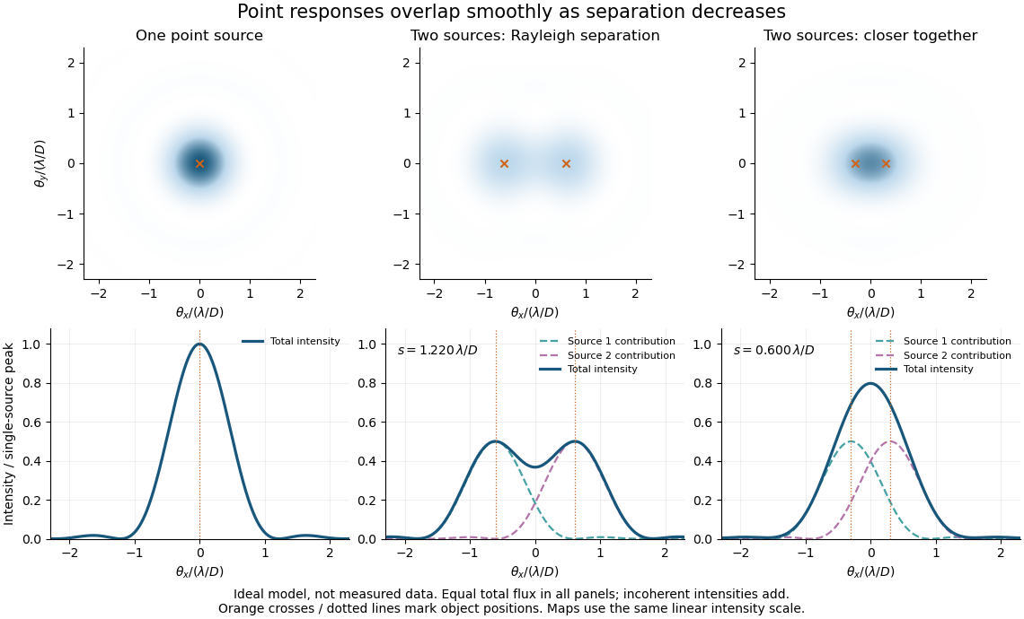
Figure 1.
Ideal circular-pupil point responses and the overlap of two mutually incoherent sources
. Details.
The figure is an original diffraction model, not measured data. All panels have the same total radiant flux: each member of a pair contributes half the single-source radiant flux. Dashed curves show the separate light intensity contributions; the solid curve is their sum. The point spread functions have tails, so even sources satisfying the Rayleigh criterion overlap. As separation decreases, the image changes continuously; there is no abrupt disappearance of all information at one separation.
A motivating measured example is Measurement of point-spread function (PSF) for confocal fluorescence microscopy by InCheon Song and others (2005). A laser, delivered through an optical fiber, excited fluorescent beads on a slide through a , numerical aperture oil-immersion objective. A moving stage scanned the bead; emitted light returned through the objective, an emission filter and a pinhole to a photodiode. The readout was fluorescence light intensity against scanned position. Under the same setup, nominal bead diameters , , and produced progressively broader measured spots. The size comparison controls for the finite object: the measured response is the convolution of bead emission with the effective point spread function, rather than a pure point response. Inverting this convolution model gave a response compared with the theoretical one. The smaller bead gave a weaker signal relative to noise; uncertainty in actual bead diameter also affected the restored width. These are limits of the calibration. In confocal microscopy, excitation and pinhole detection jointly determine the effective point spread function; this experiment does not measure the ideal widefield Airy disk plotted above.[ref]
For a new calibration, useful additional controls are to measure detector background, avoid saturating the photodetector, repeat the scan to check stability, and compare isolated beads at several positions in the field of view. Record wavelength, numerical aperture, pinhole setting, sampling interval and optical focus. These are practical recommendations, not extra measurements claimed for the published experiment.
Primordial abundances require extrapolation to material minimally processed by stars. Helium is inferred from hydrogen and helium emission in low-metallicity ionized regions, with ionization and temperature corrections. Deuterium is inferred from isotope-shifted absorption in low-metallicity quasar systems. Lithium is measured in old metal-poor stellar atmospheres and requires a correction, or a bound, for stellar depletion. These observables probe different astrophysical environments and systematic errors.
For a common semi-major axis and proper eccentricity , randomly distributed proper longitudes of periapsis give an annulus of radii and about the point displaced from the star by minus times the forced eccentricity vector, to first order in orbital eccentricity.
