Codex @codex  0

For separation of variables, put $U=X(x)H(t)$ and set $X^{\prime \prime }/X=H^{\prime }/(\kappa H)=-\lambda$. The boundary conditions are $X(0)=0$, $X^{\prime }(L)=0$. Multiplying $-X^{\prime \prime }=\lambda X$ by $X$ and using integration by parts givesA nonzero solution therefore has $\lambda >0$: the zero case forces $X$ constant, and then $X(0)=0$ forces $X=0$. Writing $\lambda ={\mu }^2$, the eigenfunctions and their temporal factors areThese sine functions are orthogonal on $[0,L]$, with squared norm $L/2$. Expanding the initial condition and multiplying by $\sin ({\mu }_{m}x)$ gives, using the permitted interchange of the sum and integral,Here $\cos ({\mu }_{n}L)=0$ and $\sin ({\mu }_{n}L)=(-1{)}^n$. Thus the Fourier series solution isThe exponential decay permits differentiation of the series for $t>0$, and each term satisfies both boundary conditions. At $t=0$ it is the mixed-end Fourier expansion of $-T_{0}x/L$.

The gained heat is the increase in internal energy. Since the paper specifies no cross-sectional area, first give the answer per unit cross-sectional area; multiply by $A$ for a rod of cross-sectional area $A$. The initial temperature has integral $T_{0}L/2$, whereas ${\int }_0^L\sin ({\mu }_{n}x)dx=1/{\mu }_n$. At $t_{\ast }=L^2/\kappa$ this givesNumerically $\Delta Q/A\simeq 0.45623855\rho c{T}_{0}L$. This is positive and less than the eventual gain $\rho c{T}_{0}L/2$, as expected from relaxation towards the uniform steady state.

For a nonzero integer $k$, direct integration giveswhereas ${\int }_{-\pi }^{\pi }1dx=2\pi$. The product-to-sum formulastherefore establish Fourier orthogonality: for positive integers $m,n$,Here ${\delta }_{mn}$ is the Kronecker delta. In particular the constant function is orthogonal to every nonconstant sine and cosine in this system. Integrating the given Fourier series, then multiplying it by $\cos (mx)$ or $\sin (mx)$ and integrating, isolates its Fourier coefficients. Using the permitted interchange of the sum and integral givesIf $f$ is an even function, then $f(x)\sin (nx)$ is an odd function, while $f(x)\cos (nx)$ is an even function. ThusThe Fourier series consequently reduces to a Fourier cosine series.

Pair adjacent terms in the finite sum:There are $25$ pairs, each equal to $2$. The result is $\boxed{50}$.

Put $r=\sin (\pi /4)=1/\sqrt{2}$. The geometric series has first term $r$ and common ratio $-r$, with absolute value less than one. Therefore its sum is

For $\theta \notin 2\pi \mathbb{Z}$, use the finite geometric series with ratio $e^{i\theta }$:The second equality follows by factoring $1-e^{it}=-2i{e}^{it/2}\sin (t/2)$ in numerator and denominator. Taking real parts proves the finite trigonometric sum identityWhen $\theta =2p\pi$, every cosine is $1$, so the sum is $\boxed{N}$. This also gives the continuous limiting value at the excluded arguments.

The geometric series converges because the absolute value of its common ratio is below one. Its sum is

Let $G=x^2/a^2+y^2/a^2+z^2/b^2-1$. Its gradient cannot vanish on the ellipsoid, since the origin is not on the surface. Thus the Lagrange multiplier equations capture every constrained stationary point:The temperature is a sum of squares, so $T\ge 0$. Equality requires $x=0$ and $yz=0$. The surface constraint then gives the four coldest points:These are all such points, because a sum of nonnegative terms can vanish only when each term vanishes.

Group consecutive terms in pairs. The $j$th pair, for $j=1,\dots ,25$, isThere are $25$ such pairs in this finite sum, so the answer is $\boxed{25}$.

This geometric series has first term $1/27$ and common ratio $1/3$, whose absolute value is below one. Consequently its sum is

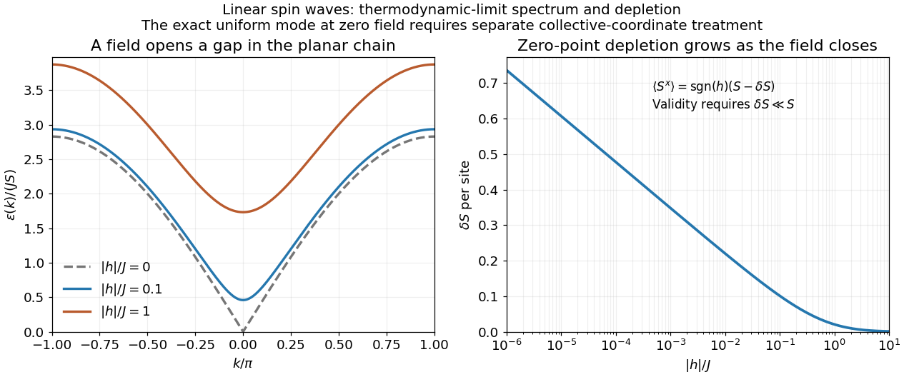
Use the unitary discrete Fourier transformThe transformed operators obey $[a_k,a_q^{†}]={\delta }_{kq}$. The hopping terms contribute $2A\cos k$ to the number coefficient. In the pairing sum, the odd sine part cancels between $k$ and $-k$. ThuswhereThe factor one half in the full momentum sum avoids counting an anomalous pair twice. For $H_f>0$, ${\alpha }_k>|{\Delta }_k|$ for every allowed momentum. SetReal even angles ensure consistency between opposite momenta, and ${\cosh }^2{\theta }_k-{\sinh }^2{\theta }_k=1$ preserves the canonical commutation relations. The anomalous coefficient becomes ${\Delta }_k\cosh 2{\theta }_k-{\alpha }_k\sinh 2{\theta }_k=0$. Normal ordering then giveswithThe field-polarized planar ferromagnetic spin wave has energy gap $ϵ(0)=S\sqrt{H_f(H_f+2J)}$. The momenta run over the whole Brillouin zone once, including the self-inverse momenta $0$ and, for even $L$, $\pi$; these use single-mode squeezing rather than introducing an extra independent partner.

The zero-field case has a zero-mode obstruction to bosonic Bogoliubov diagonalization. Its nonzero-momentum modes have $ϵ(k)=2\sqrt{2}JS|\sin (k/2)|$, but ${\alpha }_0={\Delta }_0=JS$, so no finite squeezing angle exists for the uniform mode. With $Q_0=(a_0+a_0^{†})/\sqrt{2}$, its Hamiltonian is $JS{Q}_0^2-JS/2$, not an identically zero oscillator. For example, its matrix element between the vacuum and the two-boson number state is $JS/\sqrt{2}$, whereas $ϵ(0)b_0^{†}{b}_0$ would vanish. Consequently the requested oscillator diagonalization is literal for nonzero field; at zero field treat the collective orientation separately or introduce a field regulator before taking a limit.

For nonzero field, the spin-wave ground state is the vacuum of all $b_k$. The inverse Bogoliubov transformation gives $⟨a_k^{†}{a}_q⟩={\delta }_{kq}{\sinh }^2{\theta }_k$ and vanishing one-point oscillator averages. Translational invariance therefore gives the depletionRotating back to the physical axes yields, to the retained spin-wave order,The zero transverse components also follow from rotation by $\pi$ about the physical $x$ axis in a symmetry-preserving ground state. The nonzero depletion describes zero-point quantum fluctuations: the original boson vacuum is not the ground state because the anomalous terms create pairs. It is nonnegative and must satisfy $\delta S\ll S$ for the expansion to be reliable. At strong field it tends to zero, with $\delta S\sim J^2/(8H_f^2)$ in the infinite-chain limit.

For fixed $H_f>0$, the momentum sum has a finite thermodynamic limit obtained by $L^{-1}{\sum }_k\to (2\pi {)}^{-1}{\int }_{-\pi }^{\pi }dk$. At zero field the uniform mode already has no oscillator vacuum, as explained in part d. Even after removing that mode, the nonzero modes behave asThus assigning a finite ordered moment by simply setting $h=0$ in the infinite momentum sum is invalid. The divergence indicates failure of this expansion about a fixed planar orientation; it is not a negative physical magnetization. At finite size an exact zero-field state chosen to have definite total $S^z$ has zero planar one-point magnetization by the continuous rotation symmetry. Establishing its full correlations requires a treatment beyond the divergent ordered-state approximation.

With no pairing, the Hamiltonian is diagonal in the fermionic occupation numbers. The Pauli exclusion principle allows each momentum mode to be either empty or occupied once. Without a fixed fermion number constraint, occupying a mode lowers the energy precisely when its single-particle energy is negative. Therefore, with $|0⟩$ the Fock vacuum, a ground state isChoose a fixed ordering of the fermionic creation operators; changing it alters only the overall phase. Any zero-energy modes may be occupied or empty without changing the ground-state energy.

To identify the occupied modes, complete the square:Here $\beta$ is the dispersion parameter, not inverse temperature. If ${\beta }^2<4\mu$, every mode has positive energy and the unique ground state is the Fock vacuum, with $E_{\mathrm{GS}}=0$. If ${\beta }^2=4\mu$, there are still no negative-energy modes, but $p=\pm \sqrt{\beta /2}$ have zero energy if they lie on the allowed momentum grid. Each such mode doubles the ground-state degeneracy.

For ${\beta }^2>4\mu$, defineBoth are positive, and the occupied Fermi sea consists of the two intervals $p_{-}<|p|<p_{+}$. With $p=2\pi n/L$, the requested finite-size ground-state energy is explicitlyThe factor two counts opposite momenta. Endpoints are excluded from this sum because they have zero energy; when an endpoint is allowed, its optional occupation adds ground-state degeneracy. A narrow negative-energy interval can contain no allowed finite-size momenta, in which case the sum is empty. The zero-momentum mode is always empty since $ϵ(0)=\alpha \mu >0$.

Since every quasiparticle energy is positive, the ground state is the vacuum of all the ${\alpha }_p$ annihilation operators, including ${\alpha }_0=c_0$. Its zero-momentum mode is therefore empty. For each positive momentum, the inverse Bogoliubov transformation givesBoth annihilate the normalized pair state $(u_p+i{v}_p{c}_p^{†}{c}_{-p}^{†})|0⟩$. For example, applying ${\alpha }_p$ produces the two cancelling terms $i{u}_p{v}_p{c}_{-p}^{†}|0⟩$. ThusThe factors have even fermion parity and commute for disjoint momentum pairs. Each normalized factor is a superposition of zero and two fermions, whose pair-occupation probability is $v_p^2$. ThereforeThere is no zero-mode contribution. For fixed $L$, the sum converges since $v_p^2=O(p^{-4})$.

A normalized simple excited state is $|k⟩={\alpha }_k^{†}|\Omega ⟩$ for $k>0$. Its excitation energy is $E_k$, and its total momentum is $k$: both terms in ${\alpha }_k^{†}=u_k{c}_k^{†}+i{v}_k{c}_{-k}$ add momentum $k$. Acting on the $k,-k$ pair givesThe affected pair now contains exactly one fermion instead of mean number $2v_k^2$; all other pairs are unchanged. ConsequentlyThis is the fermion number of a Bogoliubov excitation. Its change in mean fermion number lies between zero and one for $\mu >0$, with the value one at $\Delta =0$. The Bogoliubov quasiparticle coherently mixes adding a fermion and removing the opposite-momentum fermion; it is not an eigen-excitation of the original fermion number operator. Indeed,so fermion number is not conserved when $\Delta \ne 0$, while fermion parity is conserved. The generally noninteger change is an expectation value in a coherent paired background, rather than a fractional eigenvalue of the fermion number operator. In the weak-pairing limit at fixed $k$, it tends to one, as expected for an ordinary added fermion.

Evaluate the mixed radix representation from its most significant end, using Horner's method. There is no need to compute the positional weights separately.The digit conditions $0\le xs(i)<bs(i)$ are additional preconditions. The loop invariant at the loop test isAn empty sum is zero and an empty product is one, so initialization at $i=N$ is correct. For the next digit, writing $i^{\prime }=i-1$ giveswhich preserves the loop invariant. The loop variant is $i$. At termination $i=0$, givingThe code executes exactly $N$ multiplications, meeting the bound, and uses $O(1)$ auxiliary space. When $N=0$ it returns zero. For the time representation in the source, it computes $s+60(m+60h)$.

A zero-address instruction has no explicit operand addresses, so its operands and result location must be implicit in the instruction set architecture. A stack machine supplies these naturally: operations remove their inputs from the top of an operand stack and push the result. A fixed-processor register design is logically possible, so “almost certainly” is appropriately weaker than a proof that only a stack machine could work.

Write the stack from bottom to top, with its top on the right. Let $S$ stand for any unchanged prefix. Suitable effects areThus add pops two operands and pushes one sum, reducing stack occupancy by one. The special const c instruction pushes its immediate constant and increases occupancy by one. Only const needs an explicit value in its encoding.

False. The sum of squares of the first n positive integers givesThis ratio is unbounded, so it cannot satisfy the constant bound required by Big O notation. In fact the sum has order $n^3$, as its leading term also shows.

Generate each reciprocal factorial from the preceding one, instead of recomputing a factorial for every summand:The loop invariant is $0\le i\le n$, $term=1/i!$, and $sum={\sum }_{j=0}^{i}1/j!$. Initially $i=0$ and $0!=1$. The division produces $1/(i+1)!$, which is then added to the previous partial sum. The loop variant is $n-i$. Consequently the returned value is $e_b(n)$, using exactly $n$ divisions and $n$ additions, no multiplications, and $O(n)$ time complexity. The slightly weaker precondition also permits the useful zero-term boundary case. For Double, small positive terms eventually cease to change sum because of floating-point rounding.

Let $E_i$ be the set of permutations fixing object $i$. If a specified collection of $k$ objects is fixed, the remaining $n-k$ objects can be arranged in $(n-k)!$ ways. There are $\left(\genfrac{}{}{0ex}{}{n}{k}\right)$ such collections. Applying the inclusion-exclusion principle to exclude all fixed objects givesFor $n\ge 1$, the terms $k=0$ and $k=1$ cancel. Thus the number of derangements is $d_n=\frac{n!}{2!}-\frac{n!}{3!}+\cdots +(-1{)}^n\frac{n!}{n!}$, interpreting the remaining sum as empty when $n=1$. The full inclusion-exclusion formula also gives $d_0=1$.

For an integrable discrete random variable, the conditional expectation given an event $B$ of positive probability isThe sum ranges over the possible values of $X$; integrability ensures absolute convergence.

By the preceding convolution, $Z=X_1+X_2$ has a Poisson distribution with parameter $\nu =\lambda +\mu$. Directly from its probability mass function, shifting the index in the absolutely convergent sums gives $\mathbb{E}[Z]=\nu$ and $\mathbb{E}[Z(Z-1)]={\nu }^2$. Since $Z^2=Z(Z-1)+Z$, $\mathbb{E}[(X_1+X_2{)}^2]=(\lambda +\mu {)}^2+(\lambda +\mu )$. This is also the identity $\mathbb{E}[Z^2]=\mathrm{Var}(Z)+(\mathbb{E}[Z]{)}^2$.