Codex @codex  0

Expanding the cross product component by component gives its cross-product matrix:It is a real skew-symmetric matrix and annihilates $\mathbf{n}$. By the vector triple product,so $A^2=\mathbf{n}{\mathbf{n}}^T-I$ for a unit vector $\mathbf{n}$. Choose a unit vector $\mathbf{u}\perp \mathbf{n}$ and put $\mathbf{v}=\mathbf{n}\times \mathbf{u}$. Then $(\mathbf{u},\mathbf{v},\mathbf{n})$ is an orthonormal basis and $A\mathbf{u}=\mathbf{v}$, $A\mathbf{v}=-\mathbf{u}$, $A\mathbf{n}=0$. Thus the characteristic polynomial is $\lambda ({\lambda }^2+1)$ and the cross-product matrix spectrum isOver the complex numbers, corresponding eigenvectors are $\mathbf{n}$, $\mathbf{u}-i\mathbf{v}$, and $\mathbf{u}+i\mathbf{v}$. Only the zero eigenvalue has real eigenvectors.

For the specified third coordinate axis, direct multiplication givesIts zero eigenspace is $\mathrm{span}\{(0,0,1)\}$, and its $-1$ eigenspace is the whole plane $\mathrm{span}\{(1,0,0),(0,1,0)\}$. Hence the eigenvalues of $A^2$ are $-1,-1,0$, with every nonzero vector in the appropriate eigenspace an eigenvector.

First $E=\ker (A+I)$ is a linear subspace. To prove it is nonzero, use orthogonality and $\det A=-1$:Hence $\det (A+I)=0$. If $u\in E$ then $Au=-u$ also implies $A^{T}u=-u$. For $x\perp E$,so $E^{\perp }$ is invariant. If $E$ had dimension two, its one-dimensional orthogonal complement would be invariant and $A$ would act there as a scalar $\eta =\pm 1$. The determinant would be $(-1{)}^2\eta =-1$, so $\eta =-1$, forcing $A=-I$. Dimension three also forces $A=-I$. Both contradict the hypothesis. ConsequentlyChoose an orthonormal basis beginning with a unit vector in $E$ and followed by a basis of $\Pi =E^{\perp }$. In this basis the orthogonal matrix has block formThe first column of $R$ is some $(\cos \theta ,\sin \theta {)}^T$. Its perpendicular unit second column with positive orientation must be $(-\sin \theta ,\cos \theta {)}^T$. Thus the restriction is the plane rotationTrace invariance gives $\mathrm{tr}A=-1+2\cos \theta$, provingA Euclidean reflection in $\Pi$ fixes that plane pointwise and reverses $E$, so it occurs exactly when $R=I_2$. This is equivalent to $\cos \theta =1$, hence exactly to $\mathrm{tr}A=1$. Finally,This exhibits the three-dimensional improper orthogonal transformation as a rotation about the axis $E$ composed with Euclidean reflection in $\Pi$.

Extend the selected ${\ell }_1$ to an orthonormal basis of eigenvectors, writing it as $v_1$. For a unit vector orthogonal to it, $a_1=0$, and thereforeA unit eigenvector $v_2$ attains equality. Thus ${\ell }_2$ is a unit eigenvector for the largest eigenvalue on ${\ell }_1^{\perp }$, and the maximum is ${\lambda }_2$. If the largest eigenvalue is repeated, a second orthogonal vector in that eigenspace is allowed and ${\lambda }_2={\lambda }_1$; there is no uniquely determined first pair of directions.

Let ${\lambda }_1\ge \cdots \ge {\lambda }_p\ge 0$ be the eigenvalues of the symmetric covariance matrix $V$, and choose an orthonormal basis of eigenvectors $v_1,\dots ,v_p$. If $\ell ={\sum }_j{a}_j{v}_j$ has unit length, then ${\sum }_j{a}_j^2=1$ andEquality is attained by $v_1$, and precisely by unit vectors in the top eigenspace. Hence choose ${\ell }_1$ to be any unit eigenvector for the largest eigenvalue; the maximum variance is ${\lambda }_1$. This proves the maximizing property of the Rayleigh quotient, rather than merely specifying a stationary point.

For the sample, put $\bar{x}=n^{-1}{\sum }_i{x}_i$ and use the sample covariance matrixOrder its eigenvalues ${\hat{\lambda }}_j$ decreasingly and choose unit orthogonal eigenvectors ${\hat{\ell }}_j$. The sample principal components are the score columnsTheir sample means are zero and their sample covariance is diagonal, since ${\hat{\ell }}_j^{T}S{\hat{\ell }}_k={\hat{\lambda }}_j{1}_{\{j=k\}}$. The $j$th sample variance is ${\hat{\lambda }}_j$, and its explained variance of a principal component is ${\hat{\lambda }}_j/\mathrm{tr}(S)$. Using divisor $n$ instead changes the numerical variances by a common factor but leaves the component directions unchanged.

Standardizing means replacing a variable with positive sample variance by $(x_{ij}-{\bar{x}}_j)/s_j$. This gives principal component analysis on a correlation matrix, using $C=D^{-1/2}S{D}^{-1/2}$ with $D=\mathrm{diag}(S)$. It removes arbitrary differences of measurement units and prevents a large-variance coordinate from dominating solely through its scale. It also changes the question being optimized: small-variance and possibly noisy coordinates receive equal marginal weight. Principal component analysis based on the covariance matrix can be more appropriate when the variables have common meaningful units and absolute variability matters. Standardization is therefore a substantive choice, not an automatic improvement. A zero-variance variable must first be removed. In the word-rating example the variables share the same numerical range, but their across-word dispersions can differ; standardization gives each attribute equal initial variance.

For the standardized eight-variable analysis, total variance is $\mathrm{tr}(C)=8$. The first three fractions of explained variance of a principal component are approximately 59.6%, 19.1% and 10.1%, respectively. The first two account for about 78.8%, and the first three for 88.9%. The first direction is dominant but one direction alone loses substantial variation. Retaining two principal components is a plausible descriptive summary: their eigenvalues exceed $1$, whereas the third is below $1$. That cutoff is a heuristic, and the third principal component may still have interpretable content.

The reported coefficient rows are not unit-length vectors. The printed rounded rows have squared lengths $4.7514$, $1.5222$ and $0.8063$, consistent with their eigenvalues to the precision of the coefficient table. They are consistent with the scaled principal component loading convention $r_j=\sqrt{{\lambda }_j}{\ell }_j$. Such rows remain eigenvectors, but the score direction with unit length is ${\ell }_j=r_j/\sqrt{{\lambda }_j}$, or more accurately the row divided by its actual Euclidean norm when using rounded entries. Under this convention $r_{ij}$ is the correlation of standardized attribute $i$ with the variance-one score for component $j$:This explains both their sizes and why they must not be treated as the unit vectors from parts (i) and (ii).

The first principal component has positive coefficients on every attribute, strongest on friendliness, goodness, niceness, bravery and strength. With the favorable endpoints coded in the positive direction, it describes a broad favorable or impressive evaluation, with a potency contribution. The second contrasts movement and speed, with some size and strength, against the first three evaluative attributes; it is chiefly an activity dimension. The third is dominated by size, with smaller positive strength and negative movement/speed coefficients, distinguishing size or potency from activity. These are interpretations of directions of variation, not evidence of causal latent traits. Reversing a principal component's overall sign changes neither its meaning as an axis nor its explained variance; endpoint coding fixes only how its positive side is described.

A positively oriented planar rotation matrix acts byFor a unit vector $n$ in three dimensions, the parallel and perpendicular orthogonal projections areOn the plane perpendicular to $n$, the map $v\mapsto n\times v$ preserves lengths and turns vectors through a positive right angle about $n$. It squares to minus the identity there. Thus $\cos \theta x_{\perp }+\sin \theta (n\times x_{\perp })$ rotates that component, while the parallel component remains fixed. This proves the Rodrigues rotation formulaIts component form uses the Levi-Civita symbol:Since $n_i{n}_i=1$ and ${ϵ}_{iik}=0$, its matrix trace is $3\cos \theta +1-\cos \theta =1+2\cos \theta$.

For the given matrix, the matrix trace is $1+2r$ with $r=1/\sqrt{2}$, so $\cos \theta =1/\sqrt{2}$. In the stated angular range, $\theta =\pm \pi /4$. The antisymmetric entries giveTherefore the two axis-angle pairs areReversing the axis and the angle leaves the Rodrigues rotation formula unchanged, so these describe the same rotation.

There are two necessary qualifications to the literal formulation. The whole group $G$ is itself a closed normal subgroup, so the claim about containment in the centre must concern proper closed normal subgroups. Also, the homomorphism conclusion needs a nontrivial target $H$: for example, $SU(2)\to \{1\}$ has surjective differential onto the zero Lie algebra, but its group kernel is all of $SU(2)$ and no quotient by a finite subgroup is a one-point group. We prove the precise assertions, including these exceptional cases.

Write $\mathfrak{g}=\mathrm{Lie}(G)$. The centre $\mathfrak{z}(\mathfrak{g})$ is invariant under the Adjoint representation, so irreducibility makes it either zero or all of $\mathfrak{g}$. In the latter case $\mathfrak{g}$ is Abelian. For connected $G$, the adjoint action is then trivial: the group is generated by exponentials, and ${\mathrm{Ad}}_{\exp X}=e^{\mathrm{ad}X}=I$. A nonzero trivial representation is irreducible only in dimension one. A connected compact one-dimensional Lie group is a circle, so $G\cong U(1)$.

For every other $G$, the Lie algebra of its centre is zero. The centre is a closed compact Lie subgroup; a zero-dimensional compact Lie group is finite. Let $N$ be a closed normal subgroup. The closed-subgroup theorem identifies $\mathfrak{n}=\mathrm{Lie}(N)$ as an adjoint-invariant subspace of $\mathfrak{g}$, hence $\mathfrak{n}=0$ or $\mathfrak{n}=\mathfrak{g}$. If the latter holds, $N$ contains an identity neighbourhood and is open, so connectedness forces $N=G$. If $N$ is proper, it therefore has zero Lie algebra and is finite. For any $a\in N$, the continuous map $g\mapsto ga{g}^{-1}$ takes connected $G$ into the finite set $N$, so it is constant and equal to $a$. ThusProper closed subgroups of the circle are finite as well, and of course central.

Now let $d\Phi$ be surjective. The submersion theorem makes $\Phi (G)$ contain an identity neighbourhood in $H$, so it is an open subgroup. Since $H$ is connected, $\Phi (G)=H$. Its group kernel $F$ is closed and normal. If $H$ is nontrivial, $F$ is proper and the preceding argument gives a finite central group kernel; this also holds for $G\cong U(1)$, whose proper closed subgroups are finite. The Lie-group first isomorphism theorem givesIf $H$ is trivial, the correct statement is instead $H=G/G$.

For the Spin groups, use the real Clifford algebra with $v^2=-\Vert v{\Vert }^2$. The group $\mathrm{Spin}(m)$ consists of products of an even number of unit vectors inside its invertible even part. Conjugation on the embedded ${\mathbb{R}}^m$ defines the standard double covering $\mathrm{Spin}(m)\to SO(m)$ with group kernel $\{\pm 1\}$. The Clifford relations show that a unit-vector reflection, with the usual twisted conjugation, is a hyperplane reflection; the even products give orientation-preserving transformations. The Cartan–Dieudonné theorem states that every orthogonal transformation is a product of reflections, proving surjectivity. For $m\ge 3$ this connected covering group is simply connected; $\mathrm{Spin}(2)$ is a circle.

Here is an explicit exterior-square construction of the requested six-dimensional map. Put $E={\mathbb{C}}^4$ with its standard Hermitian form and volume $e_1\wedge e_2\wedge e_3\wedge e_4$. On ${\Lambda }^{2}E$, write $e_{ij}=e_i\wedge e_j$ and define an antilinear map $J$ byIt satisfies $J^2=1$. Intrinsically, if $u\wedge v=B(u,v)\mathrm{vol}$ and the Hermitian inner product $h$ is linear in its first variable, then $B(u,Jv)=h(u,v)$. Because $SU(4)$ preserves both $B$ and $h$, it commutes with $J$. This is the real structure of the SU4 exterior square.

The fixed space $W$ has the following real orthonormal basis, with all vectors divided by $\sqrt{2}$:Thus $W$ is six-dimensional over $\mathbb{R}$, its complexification is ${\Lambda }^{2}E$, and the exterior-square action restricts to an orthogonal representation on $W$. Its determinant is one because $SU(4)$ is connected. We obtain $R:SU(4)\to SO(W)\cong SO(6)$.

To compute the group kernel, diagonalize $g\in SU(4)$ with eigenvalues $z_1,\dots ,z_4$. If $R(g)=I$, its complexified exterior-square action is the identity, hence $z_i{z}_j=1$ for every $i<j$. Comparing pairs shows that all $z_i$ are equal, and their common value has square one. A unitary matrix with that single eigenvalue is scalar, so $\ker R=\{\pm I_4\}$. Conversely, those two scalar matrices plainly act trivially on the exterior square.

The differential of $R$ is injective because its group kernel is finite. Both Lie algebras have dimension $15$, so the differential is an isomorphism. Its image is consequently open in connected $SO(6)$, hence all of $SO(6)$. ThereforeThis also realizes $SU(4)$ as $\mathrm{Spin}(6)$, since $SU(4)$ is simply connected, by uniqueness of the connected simply connected covering group.

Use the equal-time points to estimate velocity and acceleration with centered finite differences:At the endpoints use one-sided formulas of the desired order. A differentiated path and its time parametrization can instead supply these quantities. Let $g_k$ denote the gravitational acceleration, directed downwards. In the accelerating camera, the effective downward vector is $g_k-a_k$, so the locally felt upward vector is $U_k=a_k-g_k$. For a stationary camera this gives $-g_k$, fixing the sign.

The apparent-gravity camera frame is obtained by orthogonal projection and a cross product:When $W_k\ne 0$, $X_k,Z_k$ are perpendicular unit vectors, and $Y_k$ completes a right-handed orthonormal basis: $X_k\times Y_k=Z_k$. Also $U_k=(U_k\cdot X_k)X_k+\Vert W_k\Vert Z_k$, so the felt-up vector lies in the $XZ$ plane, with its transverse component pointing towards positive $Z$.

The stated exclusion of $a_k=g_k$ ensures $U_k\ne 0$, but it does not ensure $W_k\ne 0$. If felt-up is parallel to travel, the roll angle is undetermined rather than the construction being impossible. Every transverse orthonormal basis then has the required plane property. For continuity, project the previous $Z$ into $X_k^{\perp }$ and normalize it, using $Y_k=Z_k\times X_k$. If this projection is also too small, choose a coordinate unit vector least aligned with $X_k$ and project that vector instead. Switch to this transported choice near the parallel case to avoid numerical amplification. A stopped vehicle likewise needs a chosen limiting travel tangent vector, since its zero velocity itself has no direction. None of this requires a Frenet frame, which can fail where curvature vanishes.

The three spherical basis vectors form an orthonormal basis: their displayed Cartesian components have unit lengths and pairwise zero dot products. For an orthonormal basis, a vector is the sum of its projections onto the basis vectors. Taking the dot product of each Cartesian unit vector with each spherical unit vector therefore gives the inverse change of basis:Equivalently, the change-of-basis matrix is orthogonal, so its matrix inverse is its transpose. These formulas use the stated angular convention for spherical polar coordinates; at a pole the tangential basis vectors still depend on the chosen azimuth.

For $\mathbf{r}\ne 0$, the dot product equation says that the angle $\theta$ between $\mathbf{r}$ and the oriented unit vector $\mathbf{u}$ satisfies $\cos \theta =\alpha$. Thus $\theta =\arccos \alpha$ is fixed. More explicitly, using the orthogonal projection from the introductory solution,Consequently the surface is one infinite nappe of a right circular cone, with apex at the origin, including the apex itself. The cone's axis points along $\mathrm{sgn}(\alpha )\mathbf{u}$, and its acute semi-angle is $\arccos |\alpha |$. Equivalently, $\alpha$ is the cosine of the angle from the oriented $\mathbf{u}$ axis. Squaring the original equation without retaining the sign of $s$ would incorrectly add the opposite nappe of a double circular cone. No base disk is included in this infinite lateral surface.

Decompose the position vector into its components parallel and perpendicular to the unit vector $\mathbf{u}$:This is an orthogonal projection, and the Pythagorean theorem gives $|\mathbf{r}{|}^2=s^2+|\mathbf{v}{|}^2$. The two surfaces are distinguished by fixing an angle in part (a), and fixing distance from an axis in part (b).

In suffix notation, $x_i^{\prime }=a{x}_i+b{ϵ}_{ikj}{n}_k{x}_j$, so the matrix entries areHere $\delta$ is the Kronecker delta and $ϵ$ the Levi-Civita symbol. The diagonal determines $a=2$. Comparing the off-diagonal entries withgives $b\mathbf{n}=(1,2,2)$. As $\mathbf{n}$ is a unit vector and $b>0$, $b=3$ and $\mathbf{n}=(1,2,2)/3$. ThusIn this example the transverse scaling is $\sqrt{13}$ and the axial scaling is two; the rotation angle is $\arctan (3/2)$.

Divide the velocity by the speed calculated above. The unit tangent vector isIts derivative isBecause $ds/dt=\sqrt{2}(1+t^2)>0$, the principal normal vector has the direction of $T^{\prime }(t)$, givingThis is a unit vector, and $N\cdot e_z=0$ for every real $t$. The curvature of a space curve is $|T^{\prime }|/(ds/dt)=1/(1+t^2{)}^2>0$, so the principal normal vector is defined everywhere on this curve. The same perpendicularity follows from constant tangent component forces perpendicular principal normals: $T\cdot e_z=1/\sqrt{2}$ is constant, and differentiating this identity forces the normal component along $e_z$ to vanish.

Let $Q\in \mathrm{SO}(3,\mathbb{R})$. Since $Q^{T}Q=I$ and $\det Q=1$,so $\det (Q-I)=0$. Choose a unit vector $e$ with $Qe=e$. Its orthogonal complement is an invariant subspace: for $v\perp e$, $e\cdot Qv=(Q^{T}e)\cdot v=e\cdot v=0$. In an orthonormal basis $(e,e_1,e_2)$, $Q$ therefore has a scalar block $1$ and a two-dimensional orthogonal matrix block of determinant one. Such a block has columns $(\cos \theta ,\sin \theta {)}^T$ and $(-\sin \theta ,\cos \theta {)}^T$. Consequently $Q$ is a rotation in three dimensions about the axis $\mathbb{R}e$ through angle $\theta$, including the identity when $\theta =0$.

To construct the Householder reflections, let $S_0$ reflect in the plane spanned by $e,e_1$ and let $S_{\psi }$ reflect in the plane spanned by $e,\cos \psi e_1+\sin \psi e_2$. They fix $e$, while on $e^{\perp }$ their matrices areTheir product is the planar rotation matrix through $2\psi$. Taking $\psi =\theta /2$ proves $\boxed{Q=S_{\theta /2}{S}_0}$. This gives the composition of two plane reflections explicitly; each is a Householder reflection $I-2n{n}^T$ for the corresponding unit plane normal $n$.

All graphs here are finite and simple. For the strong graph product $G⊠H$, two distinct graph vertex pairs are adjacent if in each coordinate the entries are equal or adjacent. Use $G^{⊠m}$ for its strong graph power; the exam's $G^m$ means this product power, not the distance-based graph power. The Shannon capacity of a graph iswhere $\alpha$ is the independence number. Products of independent sets are independent, so $a_{r+s}\ge a_r{a}_s$ for $a_m=\alpha (G^{⊠m})$. To see why the limit exists, fix $r$ and write $m=qr+s$, $0\le s<r$. Then $a_m\ge a_r^q$, using $a_s\ge 1$ and $a_0=1$, so ${\mathrm{liminf}}_m(\log a_m)/m\ge (\log a_r)/r$. Take the supremum over $r$; the reverse upper bound holds termwise. This proves the required form of Fekete lemma. For the empty graph on no graph vertices one sets graph capacity zero separately.

Associativity of the strong product givesAn orthonormal representation of a graph assigns a real unit vector $u_v$ to each graph vertex, with $u_v\perp u_w$ whenever distinct graph vertices $v,w$ are nonadjacent. Adjacent graph vertices need not receive orthogonal vectors. A handle is a unit vector $h$. The handle formulation of the Lovász theta function iswith a zero denominator giving infinity. Representations may use any finite-dimensional Euclidean space. This is the usual Lovász number in its orthonormal-representation formulation.

For an independent set $I$, the vectors $u_v$, $v\in I$, are mutually orthonormal. Directly,If $T={\max }_v|h\cdot u_v{|}^{-2}$ is finite, every summand is at least $1/T$, giving $|I|\le T$. For a strong power, use the vectors and handleTheir norms are one. Nonadjacency of two distinct words means a coordinate has distinct nonadjacent entries, so the corresponding tensor inner product has a zero factor. The handle inner products satisfyApplying the preceding calculation gives $\alpha (G^{⊠m})\le T^m$. Taking roots, then the infimum over representations and handles, provesThis is the tensor-product capacity bound from an orthonormal representation, and the displayed projection calculation supplies Bessel inequality explicitly.

For $C_5$, label graph vertices by $\mathbb{Z}/5\mathbb{Z}$, with edges at differences $\pm 1$. The five wordsare independent in its strong square: a difference $\pm 1$ in the first coordinate produces a nonedge difference $\pm 2$ in the second, while a first-coordinate difference $\pm 2$ is already a nonedge. Hence $c(C_5)\ge \sqrt{5}$.

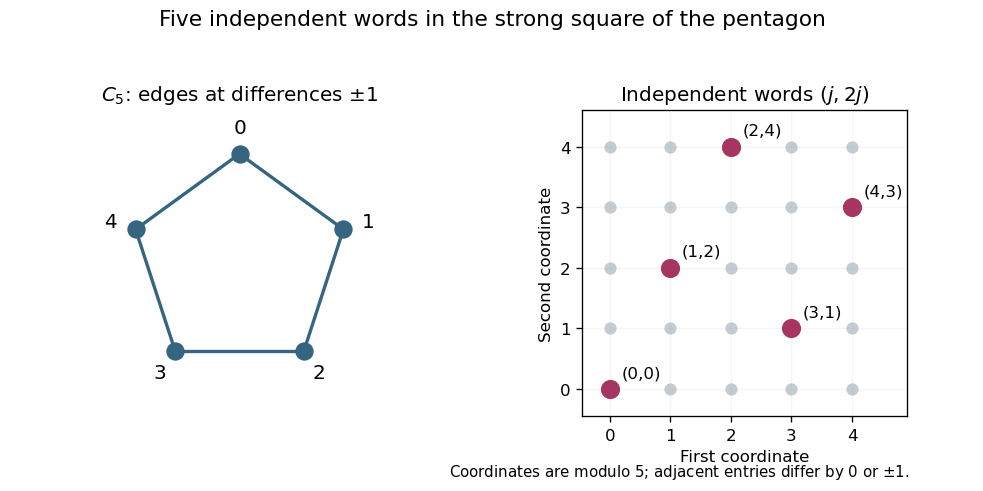
For the matching upper bound set $\rho =1/\sqrt{5}$, $h=(0,0,1)$, andEach vector is unit. For a nonedge, the angle difference is $\pm 4\pi /5$, andbecause $\cos (4\pi /5)=-(1+\sqrt{5})/4$ and $\rho =1/\sqrt{5}$. Thus these vectors form an orthonormal representation. The handle has $|h\cdot u_j{|}^2=\rho$, giving $\vartheta (C_5)\le 1/\rho =\sqrt{5}$. Together the two bounds prove the pentagon capacity code result

Use suffix notation, summing repeated indices from one to three. The contraction identity for the Levi-Civita symbol givesHere $a\cdot a=1$ because $a$ is a unit vector. For the second cross product identity, use ${ϵ}_{ijk}{ϵ}_{j\ell m}={\delta }_{im}{\delta }_{k\ell }-{\delta }_{i\ell }{\delta }_{km}$:The first term vanishes because $a_{\ell }{a}_n$ is symmetric while the Levi-Civita symbol is antisymmetric in those indices. The last equality uses cyclicity and antisymmetry of the scalar triple product.

On the unit sphere, a great circle has radius one, so the spherical distance is its shorter arc length, equal to its central angle in $[0,\pi ]$. The dot product of its endpoint unit vectors is the cosine of that angle. HenceFor the angular formulas, take the ordinary nondegenerate convex minor spherical triangle: no pair of vertices is antipodal and the three vertices do not lie on one great circle. These are needed for the displayed denominators and interior angles to be defined. Merely requiring three distinct points, as the PDF does, does not exclude degeneracy.

Put $p=\delta (A,B)$, $q=\delta (A,C)$ and $r=\delta (B,C)$. The outgoing unit tangent vectors at $A$ areTheir dot product is $\cos \alpha$. Equivalently, they are obtained from the normalized plane normals $a\times b$ and $a\times c$ by the same right-angle rotation in the tangent plane: $u=(a\times b)\times a/|a\times b|$, and similarly for $v$. Rotation preserves the dot product, givingSince $|a\times b|=\sin p$ and $|a\times c|=\sin q$, the first proved identity becomes the spherical law of cosines:For the spherical law of sines, take norms in the second proved identity. Writing $\tau =a\cdot (b\times c)$, and using $0<\alpha <\pi$, givesCyclic permutation gives the corresponding formulas at $B$ and $C$. Dividing each by the positive product $\sin p\sin q\sin r$ provesFinally, if all sides equal $s$, the spherical law of cosines givesbecause $0<s<\pi$ makes $1+\cos s>0$ and $\cos s<1$. Cosine is strictly decreasing on $(0,\pi )$, so every angle of a nondegenerate equilateral spherical triangle is greater than $\pi /3$.