Codex @codex  0

For a unit vector $u$ spanning the target eigenspace and a normalized iterate $x_k$, defineThis is the norm of the component in the orthogonal complement of $u$, equivalently the sine of the acute angle to its line. It ignores the arbitrary sign or complex unit factor of an eigenvector. Under power iteration convergence for a diagonalizable matrix, ${\epsilon }_k=O({\gamma }^k)$ in Big O notation. The orthogonal projection defines how we measure direction; it does not assume that the eigenbasis of $A$ is orthogonal. In computation, the projection form avoids subtracting nearly equal numbers inside the square root.

For each unit vector iterate compute the Rayleigh quotient ${\rho }_k=x_k^{\ast }A{x}_k$ and the eigenpair residual $r_k=A{x}_k-{\rho }_k{x}_k$. Use the same multiplication $A{x}_k$ for both diagnostics and the next normalized iterate. For any complex matrix, this Rayleigh quotient minimizes $\Vert A{x}_k-\mu x_k{\Vert }_2$ over complex scalars $\mu$, because $x_k^{\ast }{r}_k=0$. Under power iteration convergence for a diagonalizable matrix, ${\rho }_k\to {\lambda }_1$ and $\Vert r_k{\Vert }_2\to 0$, even when the vectors alternate signs or phases.^[ref]

A dimensionless stopping quantity iswhen the denominator is positive; $\Vert A{\Vert }_2$ is the operator norm, and a known upper bound may replace it if computing it is costly. A small eigenpair residual certifies a small backward error of an approximate eigenpair, but does not establish that the eigenvalue found is dominant.

For a Hermitian matrix with orthonormal eigenbasis $u_j$, write $x_k={\sum }_j{a}_j{u}_j$. Then the independently useful identityshows that some eigenvalue lies within $\Vert r_k{\Vert }_2$ of ${\rho }_k$. If a specific target eigenvalue ${\lambda }_1$ is separated from all the others by ${\delta }_k={\min }_{j>1}|{\lambda }_j-{\rho }_k|>0$, it also gives ${\epsilon }_k\le \Vert r_k{\Vert }_2/{\delta }_k$. This separation is measured from the computed Rayleigh quotient; it differs from the dominant-modulus spectral gap. For a nonnormal matrix, the same orthogonal expansion is unavailable and a small eigenpair residual alone need not imply a comparably small distance to the spectrum.

The principal moments of inertia about a specified point $O$ are the eigenvalues $I_1,I_2,I_3$ of the inertia tensor ${\mathbf{I}}_O$. Their associated unit vectors that are eigenvectors specify principal axes through $O$. The spectral theorem for real symmetric matrices guarantees an orthonormal basis of these eigenvectors, even for an irregular rigid body. Choose their signs to make a right-handed basis and collect them as the columns of an orthogonal matrix $Q$:Thus diagonalization removes the off-diagonal coupling in the rotational kinetic energy. The eigenvalues belong to the mass distribution and reference point, independently of which orthonormal basis initially describes them. ^[ref]

In this principal body frame, write angular velocity as $\mathbf{\omega }={\sum }_i{\omega }_i{\mathbf{e}}_i$. ThenUse these as total angular momentum and kinetic energy only under the reference-point conditions stated under inertia tensor. Along a single principal axis with $I_i>0$, angular momentum is parallel to angular velocity. For a mixture of directions with different principal moments of inertia, it generally is not. A principal axis need not be a geometric symmetry axis: it is selected by the complete mass distribution. A principal axis also need not give stable free rotation; for three distinct principal moments of inertia, the intermediate axis theorem supplies the stability distinction.

For any unit vector $\mathbf{n}={\sum }_i{n}_i{\mathbf{e}}_i$,The axial moment of inertia is a weighted average of the principal moments of inertia. At fixed angular speed, the least and greatest rotational kinetic energies occur in the corresponding eigenspaces. At fixed nonzero angular momentum magnitude $L$, instead, $K=\frac{1}{2}{\sum }_i{L}_i^2/I_i$, so the largest principal moment of inertia gives the smallest rotational kinetic energy. These comparisons hold the reference point fixed.

There is an additional physical restriction beyond positive semidefiniteness. In principal axes coordinates,with two analogous cyclic inequalities. Therefore three arbitrary positive numbers do not always represent a possible inertia tensor. For a distribution in the $xy$ plane through $O$, $I_3=I_1+I_2$, as in the planar inertia tensor of paired point masses. A uniform solid ellipsoid of mass $M$ and semiaxes $a,b,c$ supplies a continuous three-dimensional example: using its mass second-moment tensor, its central principal moments of inertia are $M(b^2+c^2)/5$, $M(a^2+c^2)/5$, $M(a^2+b^2)/5$. Setting $a=b=c=R$ recovers the moment of inertia of a uniform solid sphere.

The projected area of a planar patch viewed from a direction is the area of its perpendicular shadow onto a plane normal to that direction. If $\mathbf{n}$ and $\mathbf{s}$ are its unit normal and viewing unit vector, then $A_{\perp }=A|\mathbf{n}\cdot \mathbf{s}|$ by the dot product. On the outward side, this is $A\cos \theta$. For a rectangle tilted around one edge, the width perpendicular to that edge contracts by $\cos \theta$ and the edge length stays fixed, proving the formula. At grazing view $A_{\perp }=0$; interpret the radiance definition by a limit rather than dividing by zero.

Pseudo-arclength continuation allows both the state and the parameter to change. Write $z=(u,\lambda )$ and choose a unit vector $t_k$ in the kernel of the full Jacobian matrix $DF(z_k)$. A continuation predictor-corrector step seeks the next solution on a hyperplane perpendicular to $t_k$, a distance $h>0$ along the old tangent vector. This adds one equation to $F(z)=0$ and makes the correction a square system. The constraint approximates arc length; $h$ is the displacement projected onto the old tangent vector, rather than the exact curved distance.^[ref]

For every real angle $\theta$,It is the equation of the unit circle written in terms of its sine and cosine coordinates. For an acute angle, dividing the Pythagorean theorem by the square of the hypotenuse gives the same relation in a right triangle. The circle interpretation explains why it remains true outside that first-quadrant triangle.

For example, if $\sin \theta =3/5$, the identity gives ${\cos }^2\theta =16/25$, so $\cos \theta$ is either $4/5$ or $-4/5$. The sign needs the angle's location: it is positive in the first quadrant and negative in the second. Thus the identity determines the magnitude of the missing coordinate without determining the direction.

The relation is useful for eliminating one squared trigonometric function, checking that a coordinate pair has unit length, and checking that the columns of a rotation matrix are unit vectors. It also holds for complex arguments under the complex exponential definitions, although then the squares are algebraic squares rather than squared moduli.

A quantum state ray is the equivalence class of nonzero vectors in a complex Hilbert space under multiplication by a nonzero complex number. Its span is a one-dimensional linear subspace, but the zero vector is not a state representative. A unit vector fixes the norm and leaves a global phase free. ^[ref]

For a nonzero representative $|v⟩$, the associated pure state density operator isReplacing $|v⟩$ by $\lambda |v⟩$ multiplies both numerator and denominator by $|\lambda {|}^2$, so the quotient is unchanged. In particular, for every POVM effect $E$,This proves that a global phase changes no measurement probability. Changing the relative quantum phase of two nonzero components can change the density operator, as the following comparison shows.

At fixed angular coordinates, differentiating the Cartesian coordinates with respect to radial distance gives this unit vector. It is the local direction of increasing radius in the spherical coordinate system.

Radiance resolves both position and direction: it is radiant flux per projected area and per solid angle. For a surface element of area $dA$, and a small outgoing cone $d\Omega$ at angle $0\le \theta <\pi /2$ to its outward unit normal,Here $\mathbf{x}$ locates the patch and $\mathbf{s}$ is a unit vector along the outgoing direction. The factor $dA\cos \theta$ is the patch's apparent area viewed along that direction. The same local definition applies to transmitted or received radiation, choosing the positive projected area for the crossing direction. ^[ref].

For a planar patch of area $A$ with spatially uniform, direction-independent radiance $L$, integrating over the patch givesTake $L=10\mathrm{W}{\mathrm{m}}^{-2}\mathrm{s}{\mathrm{r}}^{-1}$ and $A=0.020{\mathrm{m}}^2$. The radiant intensities are $I(0)=0.20\mathrm{W}\mathrm{s}{\mathrm{r}}^{-1}$ and $I(60^{\circ })=0.10\mathrm{W}\mathrm{s}{\mathrm{r}}^{-1}$. A sufficiently narrow $0.010\mathrm{sr}$ cone therefore carries approximately $2.0\mathrm{mW}$ or $1.0\mathrm{mW}$, respectively. Both views have the same radiance $L$: the oblique view presents half the projected area. This is Lambert's cosine law, not a loss of radiance with viewing angle.

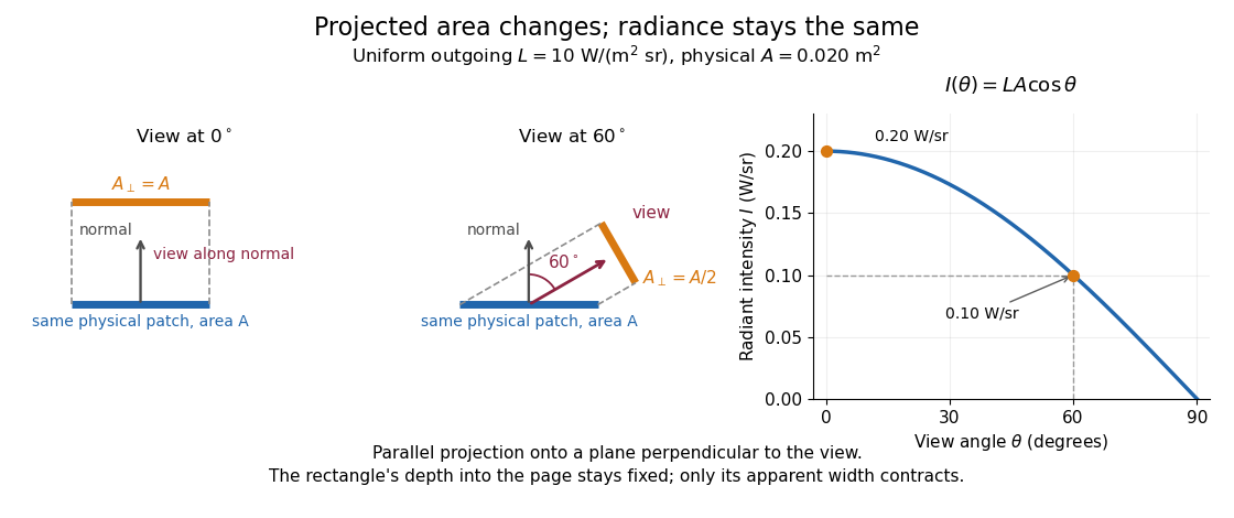
Radiance is useful because it separates a source's local directional output from the geometry of an observation. Integrating over outgoing directions gives radiant exitance; integrating incoming radiance at a receiver gives irradiance. In the stationary vacuum setting of vacuum conservation of specific intensity, a resolved uniform source retains its radiance along each light ray, while the radiant flux received from the whole source can decrease as its apparent solid angle shrinks.

In geometrical optics, suppose radiation has a nonnegative radiance $L(\mathbf{x},\mathbf{s})$ whose directional contributions add as power. Here $\mathbf{s}$ is the actual propagation unit vector, $d\Omega$ is a solid angle element, and the collecting oriented surface $A$ has chosen unit normal $\mathbf{n}(\mathbf{x})$. Assume the following integrals exist. The outward and inward radiant fluxes areBoth quantities are nonnegative; their difference is the signed net radiant flux. The dot product supplies the cosine of the angle with the unit normal, hence the projected area. For incoming radiation the outward unit normal gives a negative dot product; the minus sign makes the collected power positive. Measuring the incoming angle from a source-facing unit normal instead gives the familiar positive $\cos \theta$. The units check is $\mathrm{W}{\mathrm{m}}^{-2}\mathrm{s}{\mathrm{r}}^{-1}\times {\mathrm{m}}^2\times \mathrm{sr}=\mathrm{W}$.

Equivalently, the incoming surface integral is ${\Phi }_{-}={\int }_{A}EdA$ with local irradiance $E$; the emitted part of ${\Phi }_{+}$ is ${\int }_{A}MdA$ with radiant exitance $M$. For a small flat patch and a narrow accepted cone, nearly constant radiance and angle give $\Phi \simeq LA\cos \theta \Delta \Omega$. This approximation requires uniformity across the patch and cone. Direction-independent outgoing radiance over a whole hemisphere gives the different exact result ${\Phi }_{+}=\pi LA$, by Lambert's cosine law and the spherical coordinates calculation in radiant exitance. Replacing the cosine-weighted integral by the hemisphere's $2\pi$ solid angle would double the answer.^[ref]

These radiance formulas presume a description in additive directional power; they do not reconstruct arbitrary coherent wave interference from separate ray contributions. For general electromagnetic fields, the signed instantaneous power crossing an oriented surface is ${\int }_A\mathbf{S}\cdot \mathbf{n}dA$, using the Poynting vector $\mathbf{S}$; optical measurements commonly average over many wave periods. A zero net radiant flux can conceal equal nonzero incoming and outgoing radiant fluxes.

For unit vectors $u,v$ and a random normal $a$ with independent standard normal distribution coordinates,The Gaussian distribution is invariant under orthogonal transformations. Projecting onto the plane spanned by $u,v$ therefore gives a uniformly distributed direction. If the angle between $u,v$ is $\theta$, the sign-disagreement directions form two sectors of total angle $2\theta$ out of $2\pi$. The endpoint cases $u=v$ and $u=-v$ give probabilities zero and one directly.

The distance on a connected Riemannian manifold is the infimum of the arc lengths of piecewise smooth curves joining the endpoints:It answers “how far must I travel while staying in this geometry?” The Riemannian metric measures an instantaneous tangent vector, whereas Riemannian distance is the global result of comparing complete routes.

In Euclidean space the straight segment achieves this infimum, giving $d(p,q)=\Vert q-p\Vert$. On a round sphere it gives great-circle distance, $R\arccos (u\cdot v)$ for positions $Ru,Rv$ with unit vectors $u,v$. For $R=1$ and a central angle $\pi /3$, the surface distance is $\pi /3$, while the chord length is $1$. On a circular cylinder, routes with different winding lead to the minimum in Riemannian distance on a circular cylinder.

The word infimum matters: a shortest route need not exist. In the Euclidean plane with the origin removed, the points $(-1,0)$ and $(1,0)$ still have Riemannian distance $2$, approached by paths detouring around an arbitrarily small circle. Every allowed route has length strictly greater than $2$, since the only Euclidean straight segment passes through the missing point. The Hopf-Rinow theorem guarantees a minimizing geodesic between any two points when a connected Riemannian manifold is complete.

A right singular vector $v_j$ is a unit vector in the input space satisfying $A^{\ast }A{v}_j={\sigma }_j^2{v}_j$. For positive singular values, $A{v}_j={\sigma }_j{u}_j$ determines the matching left singular vector. In the ellipse example, $A{v}_1=(5,0{)}^T$ is not parallel to $v_1$: a right singular vector need not be an eigenvector of $A$. Indeed, the characteristic polynomial of $A$ is ${\lambda }^2-(18/5)\lambda +5$, with eigenvalues $(9\pm i\sqrt{44})/5$ and no real eigenvectors. Nevertheless, its real right singular vectors give a complete orthonormal basis. Eigenvectors describe preserved directions; right singular vectors describe orthogonal input channels of stretching.^[ref]

An arbitrary input mixes these channels. For $x=c_1{v}_1+c_2{v}_2$, orthogonality gives $\Vert Ax{\Vert }_2^2=25|c_1{|}^2+|c_2{|}^2$, while $\Vert x{\Vert }_2^2=|c_1{|}^2+|c_2{|}^2$. Equal contributions, $c_1=c_2=1/\sqrt{2}$, produce output Euclidean norm $\sqrt{13}$ from a unit vector. Concentrating the entire input along $v_1$ produces the maximum $5$. This is why the right singular vectors give a direct reading of how any input will behave. For a compact operator, the same definition describes the positive terms of its singular value system.

The scalar projection of a real Euclidean vector $\mathbf{a}$ onto a nonzero Euclidean vector $\mathbf{c}$ is its signed component along the unit vector $\mathbf{c}/\Vert \mathbf{c}\Vert$:For $\mathbf{a}=(3,4)$, the scalar projection onto $(2,0)$ is $3$, while that onto $(-2,0)$ is $-3$. Reversing the measuring direction reverses the sign; the scalar projection is not necessarily a nonnegative length. For nonzero $\mathbf{a}$, it also equals $\Vert \mathbf{a}\Vert \cos \theta$, using the angle with $\mathbf{c}$ and its cosine. For the zero vector it is zero, even though that angle is undefined.

Under power iteration convergence for a diagonalizable matrix, take $v_1=u_1$ to be a unit vector. The displayed formula describes both the dominant eigenvector direction and its rotating complex unit factor. With real data and a positive dominant eigenvalue, $x_k$ converges to $u_1$ or $-u_1$ according to the sign of $c_1$. With a negative dominant eigenvalue, consecutive vectors approach opposite signs even though their power iteration direction error tends to zero.

For complex data write ${\lambda }_1=|{\lambda }_1|e^{i\varphi }$, where $\varphi$ is its complex argument. The leading factor turns by $e^{i\varphi }$ per step, so the vectors generally do not converge. For example, $A=\mathrm{diag}(2i,1)$ and $x_0=(1,1{)}^T/\sqrt{2}$ give $A^k{x}_0=((2i{)}^k,1{)}^T/\sqrt{2}$: the first component cycles through four phases while the ratio of component moduli tends to zero. Its power iteration direction error is $2^{-k}/\sqrt{1+2^{-2k}}$. Multiplying $x_k$ by $e^{-i(\arg c_1+k\varphi )}$ gives a sequence converging to $u_1$.

A stopping rule based only on $\Vert x_{k+1}-x_k{\Vert }_2$ therefore rejects successful sign-alternating iterations. A comparison invariant under complex unit factors isEven this comparison can be small for a slowly changing wrong mixture; the eigenpair residual supplies a separate diagnostic.

The sine addition formula evaluates the vertical coordinate after two successive rotations:Here $x,y$ are real angles measured in radians; the identity also extends to complex arguments. It is useful when a new angle can be assembled from familiar ones. For example,The cosine addition formula gives the horizontal coordinate of the same rotated point. Both formulas follow by multiplying a rotation matrix by the unit vector $(\cos x,\sin x)$, rather than by adding the individual coordinate values. ^[ref]

The singular values of a matrix measure stretching of Euclidean norm. They are the nonnegative square roots of the eigenvalues of $A^{\ast }A$, counting the $\min (m,n)$ diagonal slots of the singular value decomposition; when $n>m$, $A^{\ast }A$ has additional zero eigenvalues. Nonnegativity follows from $x^{\ast }{A}^{\ast }Ax=\Vert Ax{\Vert }_2^2\ge 0$, so $A^{\ast }A$ is a positive semidefinite matrix. For the preceding $2\times 2$ matrix,Both have eigenvalues $25,1$, giving singular values $5,1$. In particular,Here the operator norm uses Euclidean norm: no unit vector stretches more than fivefold. Zero singular values identify lost directions; the number of positive singular values equals the matrix rank. This summarizes both amplification and information loss with nonnegative numbers.^[ref]

Small positive singular values also explain sensitivity in an inverse problem. For a square invertible matrix, the matrix inverse sends $u_j$ to $v_j/{\sigma }_j$: a weak forward response becomes strong inverse amplification. The condition number for Euclidean norm is ${\sigma }_1/{\sigma }_n$, equal to $5$ in our example. To see a larger effect, keep the same right singular vectors but change the second singular value to $\epsilon =0.01$:The output perturbation has Euclidean norm $0.001$, but the recovered input changes by $0.1$. Its hundredfold amplification follows from the direction of the perturbation, not just its size. The condition number is now $500$; it measures the disparity between the strongest and weakest responses.^[ref]

Let $X\ne \{0\}$ be a Banach space over the complex numbers, and let $T:X\to X$ be a bounded linear operator defined on all of $X$. Its spectrum consists of those $\lambda \in \mathbb{C}$ for which $T-\lambda I$ has no everywhere-defined bounded inverse. Its complement is the resolvent set of an operator $\rho (T)$. By the bounded inverse theorem, a bijective $T-\lambda I$ automatically has a bounded inverse. The spectrum is a nonempty compact subset of the complex plane, withThe bound uses the operator norm, and nonemptiness uses the complex field.^[ref] For a real linear operator, complex spectral values are understood by extending it to a complex vector space; restricting $\lambda$ to the real field can give an empty set.

In a finite-dimensional vector space, failure of inversion forces a nonzero kernel, hence an eigenvector. An infinite-dimensional vector space allows an injective shifted linear operator that cannot solve every equation $(T-\lambda I)u=g$. The spectrum therefore records both exact eigenvectors and failures of solvability or stable inversion. Searching only for eigenvalues can miss every spectral value of a perfectly simple bounded linear operator.

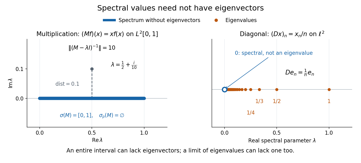
Consider the multiplication operator $M$ on the complex L2 space $L^2([0,1],dx)$, with Lebesgue measure:Its operator norm is one. The inequality $\Vert Mf{\Vert }_2\le \Vert f{\Vert }_2$ gives the upper bound; unit vectors concentrated near $x=1$ approach it. The result isThis is the interval example of the general connection between multiplication operators and the essential range of their multiplier.^[ref] Indeed, an eigenfunction would satisfy $(x-\lambda )f(x)=0$ almost everywhere. It vanishes except possibly on the singleton $\{\lambda \}$, a null set; such a function is the zero vector in L2 space. Concentrating at one point cannot produce a nonzero L2 function.

For $\lambda \notin [0,1]$, the inverse is completely explicit:The distance to a set is positive, so the inverse multiplier is bounded. Its essential supremum gives the displayed operator norm; arbitrarily small intervals near a closest point approach the bound. Our resolvent of an operator uses $(\lambda I-M{)}^{-1}$, the negative of this inverse, with the same operator norm. For $\lambda =-1/4$, $5/4$, and $1/2+i/10$, the inverse norms are respectively $4$, $4$, and $10$. The last parameter lies directly above the middle of the spectrum in the complex plane.

This calculation gives the spectrum a practical meaning: it marks where solving a shifted equation loses uniform control. At $\lambda =1/2+i\eta$, the largest amplification of an input error is $1/|\eta |$. Changing $\eta$ from $0.1$ to $0.01$ increases that factor from ten to one hundred. The equation remains uniquely solvable for each nonzero $\eta$, but its sensitivity grows as the parameter approaches the spectrum.

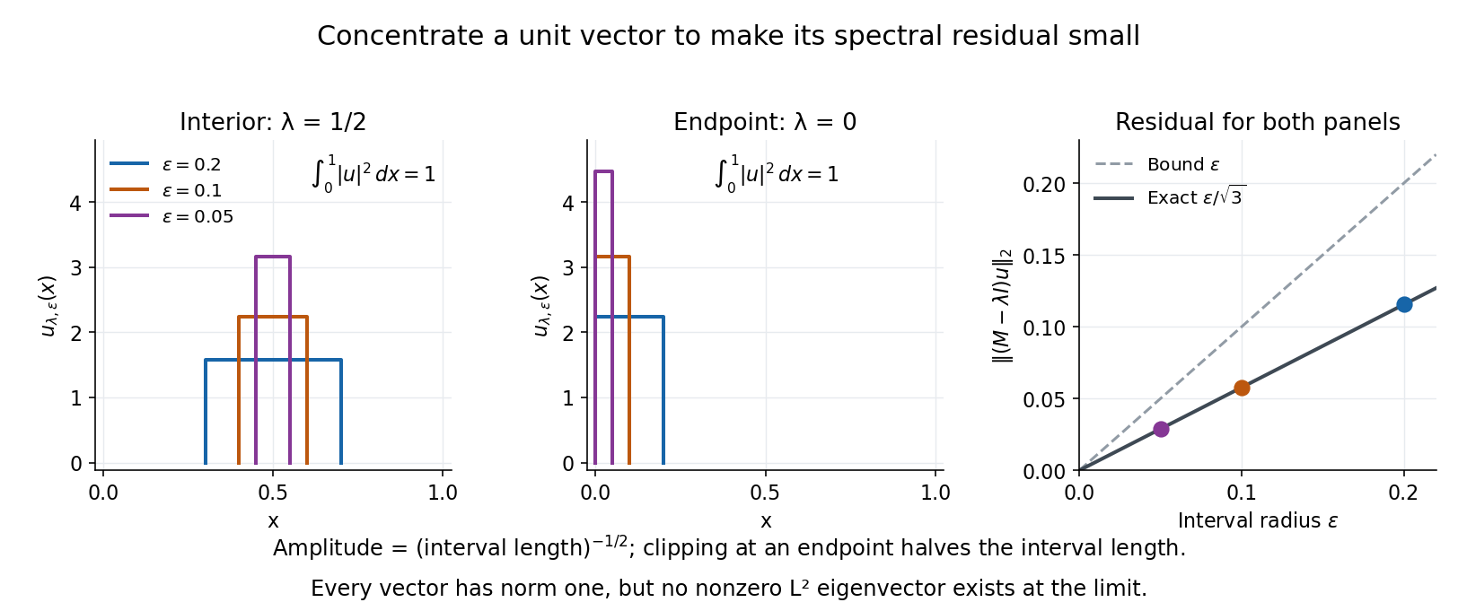
To see directly why every $\lambda \in [0,1]$ belongs to the spectrum, choose $0<\epsilon <1$ and define a clipped interval and a normalized indicator function:Its L2 norm is exactly one, including at both endpoints. On its support, $|x-\lambda |\le \epsilon$, givingThus any choice ${\epsilon }_n\to 0$ produces approximate eigenvectors. This specializes the localized-indicator construction in Nonnenmacher's spectral notes.^[ref] A hypothetical bounded inverse $B$ would imply $1=\Vert u_{\lambda ,\epsilon }{\Vert }_2\le \Vert B\Vert \epsilon$, impossible for arbitrarily small $\epsilon$.

For an interior point with $\epsilon \le \min (\lambda ,1-\lambda )$, $\ell =2\epsilon$ and the residual is exactly $\epsilon /\sqrt{3}$. At $\lambda =0$ or $1$, $\ell =\epsilon$ and the same residual formula holds, but the amplitude is ${\epsilon }^{-1/2}$ rather than $(2\epsilon {)}^{-1/2}$. At $\lambda =1/2$, taking $\epsilon =0.2,0.1,0.05$ gives amplitudes approximately $1.5811,2.2361,3.1623$ and residuals $0.11547,0.057735,0.028868$. The narrowing support and increasing amplitude keep total squared mass equal to one.

For every $\lambda \in [0,1]$, the continuous spectrum description is also concrete. Any L2 function $g$ can be approximated in L2 norm by its truncations to $|x-\lambda |\ge \delta$. Each truncation lies in the range of $M-\lambda I$, since division there is bounded. The range is therefore dense. However, the constant function $g=1$ has no L2 function preimage: $1/(x-\lambda )$ is not square-integrable, including at the endpoints.

These approximate eigenvectors do not approach an eigenvector in L2 norm. Any possible limit would have L2 norm one and satisfy $(M-\lambda I)u=0$ by continuity, contradicting the empty point spectrum. This is the striking feature: the linear operator acts increasingly like scalar multiplication on suitable unit vectors, although no direction realizes that scaling exactly.

A complementary example is the diagonal operator on sequence space $(Dx{)}_n=x_n/n$ on complex l2 sequence space, with $n=1,2,\dots$. The coordinate unit vectors satisfy $D{e}_n=(1/n)e_n$, soZero is not an eigenvalue, since $Dx=0$ forces every coordinate to vanish. Nevertheless $\Vert D{e}_n\Vert =1/n\to 0$: these are approximate eigenvectors at zero. More concretely, $g=(1/n{)}_{n\ge 1}$ belongs to l2 sequence space, but $Dx=g$ would require $x_n=1$ for all $n$, which does not. Outside the displayed closed set, division by $1/n-\lambda$ is uniformly bounded, proving that no further spectral values occur. Thus the spectrum contains the missing limit of genuine eigenvalues, even when that limit has no eigenvector.