Codex @codex  0

Using $BA=AB$ and linearity,This establishes that commuting maps preserve eigenspaces. The vector $Av$ can be zero, so this step alone does not assert that $Av$ is an eigenvector.

Work over the field containing the stated $n$ distinct eigenvalues of $B$; in a real formulation these must be real to obtain real eigenvectors. Choose one eigenvector for each distinct eigenvalue. By independence of eigenvectors for distinct eigenvalues, these $n$ vectors are a basis. Consequently each eigenspace $E_{\lambda }(B)$ has dimension one: in an expansion in this eigenbasis, $Bw=\lambda w$ forces every coefficient with a different eigenvalue to vanish.

Now let $v\ne 0$ be any eigenvector of $B$. By part (d), $Av$ belongs to its one-dimensional eigenspace, so $Av=\mu v$ for some scalar $\mu$. This proves that $v$ is an eigenvector of $A$, including the case $Av=0$, where $\mu =0$. This is the crucial one-dimensional step in simple spectrum gives simultaneous diagonalization.

Every output $u_1+u_2$ lies in the sum of subspaces $W_1+W_2$, since it is a linear combination of members of the two vector subspaces. For $u=(u_1,u_2)$, $v=(v_1,v_2)$ and scalars $a,b$,Therefore $g$ is a linear map. Every vector in $W_1+W_2$ is such an output: group the terms of any linear combination from $W_1\cup W_2$ according to their originating vector subspace. Thus the addition map of subspaces is also surjective.

The kernel of a linear map $g$ is precisely $U$, sincePart (c) gives $\mathrm{im}g=W_1+W_2$. Apply the rank-nullity theorem to the finite-dimensional vector space $W_1\times W_2$, and then parts (a) and (b):This proves the dimension formula for a sum of subspaces. The kernel of a linear map records exactly the freedom to transfer a shared vector from one summand to the other without changing their sum.

The gradient vanishes at $0$. Decompose any vector as $x=tb+w$, with $w\perp b$. Symmetry of $A$ and $Ab=\frac{1}{2}b$ imply $b^{T}Aw=(Ab{)}^{T}w=0$. Since $\Vert b\Vert =1$,If $d\ge 2$, choose a nonzero $w\perp b$. Arbitrarily close to zero, the direction $b$ gives negative values and the direction $w$ gives positive values. Thus $0$ is a saddle point for $d\ge 2$. Equivalently, the Hessian matrix has one negative eigenvalue and all its other eigenvalues positive.

The dimension matters: if $d=1$, the orthogonal complement is zero-dimensional and $g(tb)=-t^2/2$. In that case $0$ is the unique global maximum. This edge case is not excluded by the stated hypotheses. The decomposition is a rank-one downdate along an eigenvector.

If $A^{\top }x=0$, the vector $x$ belongs to the null space for which the columns of $L$ are a basis. It is therefore a linear combination of those columns, so $x=Ly$ for some $y\in {\mathbb{R}}^m$. Conversely, each column is annihilated by $A^{\top }$, hence $A^{\top }L=0$ and $x=Ly$ implies $A^{\top }x=0$. ThusThe coordinate vector $y$ is unique because the columns of $L$ are linearly independent.

Fix one common eigenvector $v\ne 0$, and write $A{A}^{\top }v=\lambda v$ and $B{B}^{\top }v=\mu v$. By (d),so $\lambda \mu v=0$ and at least one of the two eigenvalues is zero.

To exclude both being zero, use the kernel of a Gram product identity:If both products annihilate $v$, then $A^{\top }v=B^{\top }v=0$. By (b), $v\in \mathrm{im}L$, and by (e), this is $\mathrm{im}B$. On the other hand, $B^{\top }v=0$ makes $v$ orthogonal to every vector in $\mathrm{im}B$. In particular $v$ is orthogonal to itself, so $\Vert v{\Vert }^2=0$ and $v=0$, a contradiction.

Therefore each specified common eigenvector belongs to exactly one of $\ker (A{A}^{\top })$ and $\ker (B{B}^{\top })$. Both eigenvalues are nonnegative by the displayed squared-norm identities, so the other eigenvalue is strictly positive. This is the spectral mechanism behind orthogonal null-space completion of a square matrix.

If $A$ is a skew-symmetric matrix, the scalar $x^{\top }Ax$ equals its own transpose, soand it is zero over the real numbers.

Conversely, suppose the quadratic form $x^{\top }Ax$ vanishes for every real vector. Substituting $x=e_i$ gives $a_{ii}=0$. Substituting $x=e_i+e_j$ gives $a_{ij}+a_{ji}=0$ for $i\ne j$. Therefore $A^{\top }=-A$. This proves the quadratic-form criterion for a skew-symmetric matrix:

For the product order, reflexivity follows from $a_i\le a_i$ in every coordinate. If $\mathbf{a}⪯\mathbf{b}$ and $\mathbf{b}⪯\mathbf{a}$, the antisymmetric relation axiom for the usual real order gives $a_i=b_i$ for every $i$, hence $\mathbf{a}=\mathbf{b}$. If $\mathbf{a}⪯\mathbf{b}⪯\mathbf{c}$, transitivity in each coordinate gives $a_i\le c_i$, hence $\mathbf{a}⪯\mathbf{c}$. Thus this is a partial order.

For $n\ge 2$, the vectors $(1,0,0,\dots )$ and $(0,1,0,\dots )$ are incomparable: each has a coordinate larger than the corresponding coordinate of the other. It is not a total order for $n\ge 2$. The dimension qualification matters: for $n=1$ this is the usual total order on $\mathbb{R}$, so the printed non-totality claim needs the implicit assumption $n\ge 2$.

Interpret the norms as Euclidean norms and set $B=A^{\mathsf{T}}A$. This is a real symmetric matrix with ${\mathbf{x}}^{\mathsf{T}}B\mathbf{x}=\Vert A\mathbf{x}{\Vert }^2\ge 0$, hence a positive semidefinite matrix. Squaring the nonnegative objective does not change its argmin. Let ${\lambda }_{\min }$ be the smallest eigenvalue of $B$ and $E_{\min }$ its eigenspace.

First minimize on the unit sphere. The Lagrange multiplier function $L(\mathbf{x},\lambda )={\mathbf{x}}^{\mathsf{T}}B\mathbf{x}-\lambda ({\mathbf{x}}^{\mathsf{T}}\mathbf{x}-1)$ has stationarity condition $B\mathbf{x}=\lambda \mathbf{x}$. Multiplication by ${\mathbf{x}}^{\mathsf{T}}$ shows that the squared objective at such a point is $\lambda$. The spectral theorem for real symmetric matrices also gives, for every unit vector, ${\mathbf{x}}^{\mathsf{T}}B\mathbf{x}\ge {\lambda }_{\min }$, with equality exactly in $E_{\min }$. This proves global minimality, rather than merely finding stationary candidates.

If ${\lambda }_{\min }>0$, every point with $\Vert \mathbf{x}\Vert >1$ has a strictly smaller objective after rescaling to unit length. ThereforeIf ${\lambda }_{\min }=0$, the kernel of a linear map satisfies $\ker B=\ker A$, since $B\mathbf{x}=0$ implies $\Vert A\mathbf{x}{\Vert }^2=0$, and the converse is immediate. The minimum is then zero, attained precisely atIn this case minimizers need not have unit length. This distinction is essential for a rank-deficient $A$, including any real $m\times n$ matrix with $m<n$. The result is the minimum image norm outside a Euclidean unit ball, governed by the least singular value.

Put $h=\Delta x$ and suppose $L=(n+1)h$, so there are $n$ interior grid points $x_j=jh$, $j=1,\dots ,n$. Write $u_j(t)\simeq u(x_j,t)$. The fixed ends impose homogeneous Dirichlet boundary conditions,For a sufficiently smooth displacement field, the two Taylor series at fixed time givewhere all displayed derivatives on the right are evaluated at $(x_j,t)$. Adding cancels the odd terms, leaving the second-order central differenceSubstitute this finite difference into the wave equation and retain continuous time. The resulting method of lines gives coupled second-order ordinary differential equations,In particular, the first and last equations are ${\ddot{u}}_1=(c^2/h^2)(-2u_1+u_2)$ and ${\ddot{u}}_n=(c^2/h^2)(u_{n-1}-2u_n)$ for $n\ge 2$. With the interior displacement vector only,Equivalently, $A_{jj}=-2c^2/h^2$, $A_{j,j+1}=A_{j+1,j}=c^2/h^2$, and all other entries vanish. This entrywise definition also covers small $n$, including $A=(-2c^2/h^2)$ when $n=1$. The matrix is a symmetric matrix and a tridiagonal matrix. The spatial approximation has error $O(h^2)$ in Big O notation; time has not yet been discretized.

For a nonzero, time-independent vector $\hat{\mathbf{u}}$, substitute $\mathbf{u}(t)=\hat{\mathbf{u}}{e}^{i\omega t}$. Taking two time derivatives givesCancel the nonzero exponential to obtain the eigenvalue problemThus an eigenvector specifies a normal mode shape and its negative eigenvalue specifies the square of its angular frequency, $\omega =\sqrt{-\lambda }$. Real displacements are obtained by taking the real part, or by combining the two temporal solutions as $\hat{\mathbf{u}}(a\cos \omega t+b\sin \omega t)$.

For each row, a Gershgorin disc has centre $a_{jj}=-2$ and radius $r_j={\sum }_{k\ne j}|a_{jk}|$. Here $r_1=r_3=1$ and $r_2=2$, so the Gershgorin circle theorem givesSince $A$ is a real symmetric matrix, its eigenvalues are real. Intersecting the union of these Gershgorin discs with the real axis yieldsThis bound permits zero but does not assert a zero eigenvalue. The fixed-end Dirichlet boundary conditions exclude it: for any nonzero real vector $v=(v_1,v_2,v_3{)}^T$, extend by $v_0=v_4=0$ and calculateIndeed, equality would force every adjacent value to agree with the zero endpoint. Thus $-A$ is a symmetric positive-definite matrix, $A$ is a negative-definite matrix, and the eigenvalues satisfy $-4\le \lambda <0$. The same argument works for any number of interior grid points, with prefactor $c^2/h^2>0$ in the sum. The fixed string has no zero-frequency rigid translation.

Each supplied eigenvector gives relative displacements at $x=1,2,3$ in a standing wave. Insert zero at $x=0,4$ to describe the whole sampled string. A real normal mode is $u_j(t)=C{v}_j\cos (\omega t+\varphi )$: its shape stays fixed while its amplitude oscillates.

These semidiscrete fixed-string normal modes are samples of $\sin (k\pi x/4)$, with $k=3,2,1$ in the order listed. More precisely, their interior vectors are $v_j^{(k)}=2^{-1/2}\sin (k\pi j/4)$, which have unit Euclidean norm and form an orthonormal basis of ${\mathbb{R}}^3$. Their eigenvalues and angular frequencies obeyThus larger absolute value of a negative eigenvalue means faster oscillation, rather than faster decay. The numerical angular frequencies approximate the continuous fixed-string values $k\pi c/L$; the finite difference spatial approximation changes them. Only three independent interior normal modes exist on this grid, and any interior displacement or initial velocity vector can be expanded in this orthonormal basis.

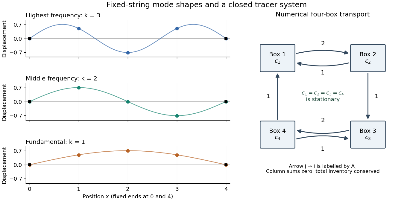
Regard $A$ as a linear map ${\mathbb{R}}^4\to {\mathbb{R}}^4$. By the rank-nullity theorem and matrix rank $3$,All three are vector subspaces of ${\mathbb{R}}^4$, with the row space identified with four-component row vectors in the usual way. The null space lies in the input vector space of concentrations; the column space lies in the output vector space of concentration-change rates. Both have four coordinates, although they play different physical roles.

In this particular matrix, the row sums and column sums both vanish. Put $1=(1,1,1,1{)}^T$. Then $A1=0$ and $1^{T}A=0$, and the two three-dimensional vector subspaces coincide:This equality follows here from both sum identities and the dimensions of a vector space; it does not make $A$ a symmetric matrix and is not true for every square matrix.

The null space consists of concentration patterns on which transport produces no change. Here it is the familyEvery box has the same concentration. Ocean circulation may continue, but inflow and outflow of the chemical tracer balance in each box. With $\mathbf{b}=0$ these are exactly the steady states; physically admissible members have $\alpha \ge 0$. With nonzero $\mathbf{b}$, adding $\alpha 1$ to any particular steady state leaves its transport balance unchanged, but a null space vector alone need not balance the sources and sinks.

To identify the tracer inventory, apply conserved inventory from a left null vector. Directly summing each column givesConsequently, for the supplied ordinary differential equations,For $\mathbf{b}=0$, $M$ is a conserved quantity. The connected box model equalizes concentrations, approaching the unique member of the null space with the initial inventory:The arithmetic mean is appropriate here because the supplied matrix has zero column sums. In a general box model the conserved quantity is $w^T\mathbf{c}$, where $w$ is a positive left null space vector; for physical concentrations expressed per unit volume, these weights represent the box volumes up to a common factor. One must establish the weights from the equations, rather than infer equal volumes from a schematic drawing.

Nonnegative initial concentrations remain nonnegative under transport alone. Indeed $A+2I$ is a nonnegative matrix, sohas nonnegative entries for $t\ge 0$: it is a positive matrix semigroup. Its column sums are one by $1^{T}A=0$. To see why equalization occurs, set $d=\mathbf{c}-(M/4)1$ for $\mathbf{b}=0$; then $1^{T}d=0$ andThe right side vanishes only for constant $d$, which in the zero-sum vector subspace means $d=0$. Its strict negative bound on the unit sphere in that vector subspace gives decay to zero. Thus the matrix exponential redistributes inventory without creating negative concentrations; arbitrary prescribed sinks can still exhaust the tracer if they are allowed to act indefinitely.

A steady state ${\mathbf{c}}_{\ast }$ satisfies $0=A{\mathbf{c}}_{\ast }-\mathbf{b}$, henceThe sign is positive on the right after rearranging the supplied equation. A solution exists exactly when $\mathbf{b}$ lies in the column space of $A$, which above was found to be the zero-sum vector subspace. Equivalently, multiply by the left null space vector $1^T$:This condition is necessary and sufficient for an algebraic steady state, since both the column space and that zero-sum vector subspace have dimension $3$. It expresses global conservation of mass: in the closed box model, total tracer production must balance total tracer removal. With the paper's convention $-\mathbf{b}$, a positive $b_i$ is a sink and a negative $b_i$ is a source. If the sum is nonzero, $dM/dt=-{\sum }_i{b}_i$ and the inventory changes linearly in time, preventing a steady state.

When the condition holds, all algebraic steady states form the affine solution space of a linear equation ${\mathbf{c}}_p+\alpha 1$, for any particular solution $A{\mathbf{c}}_p=\mathbf{b}$. The initial inventory selects one member through $1^T{\mathbf{c}}_{\ast }=1^T\mathbf{c}(0)$. For a physically admissible solution, its four concentrations must additionally be nonnegative; the compatibility condition alone imposes no such inequalities.

Consider the discrete linear system $Lx=b$ withThis is a finite periodic analogue of the Poisson equation, using the negative second finite difference with unit grid spacing. It is also a Graph Laplacian equation on a cycle graph; no continuum approximation is being claimed here.

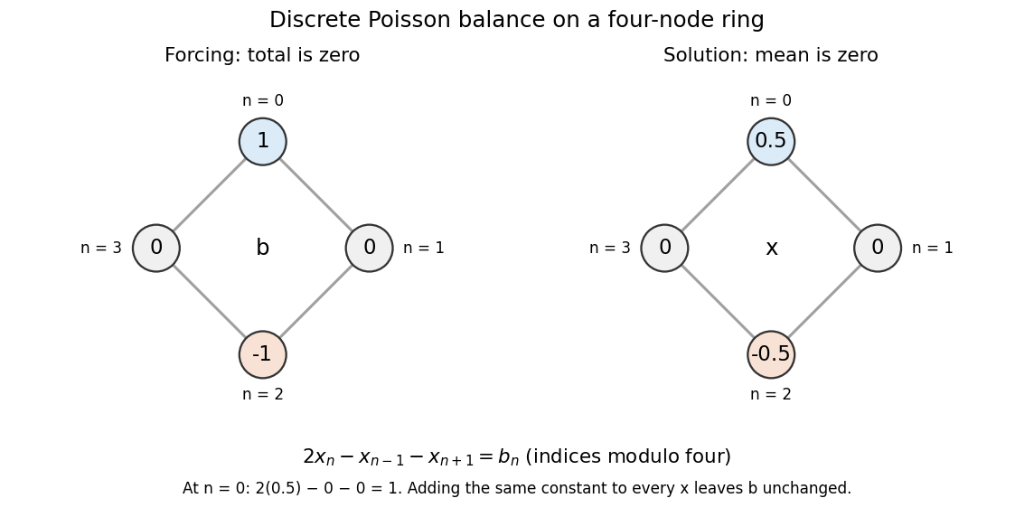
Summing the four equations gives zero on the left, since each value occurs twice positively and twice negatively. A necessary condition is therefore ${\sum }_n{b}_n=0$. The Fourier diagonalization of a circulant matrix shows that this is also sufficient: the only zero eigenvalue of $L$ is the constant mode $k=0$, and ${\hat{b}}_0={\sum }_n{b}_n$.

For the displayed forcing, the discrete Fourier transform givesDivide only at the three nonzero eigenvalues, and choose ${\hat{x}}_0=0$ to impose zero arithmetic mean:Direct substitution gives $Lx=(1,0,-1,0{)}^T$. All other vectors satisfying the linear system are $x+a(1,1,1,1{)}^T$, because the kernel is the space of constant vectors. Thus balanced forcing determines the differences between values, while a reference level is an extra choice. This small model explains why a periodic Poisson equation needs both a compatibility condition and a normalization.

A vector describing direct selection on measured phenotypic traits, conditional on the other measured traits. In a local deterministic fitness model it can be written $\mathbf{\beta }={\nabla }_{\mathbf{z}}\log w$; population regression estimates require their own sampling and fitness assumptions. This differs in context from a rare-mutant invasion selection gradient.

Absorption of momentum $\mathbf{p}$ followed by emission of ${\mathbf{p}}^{\prime }$ changes a free atom's momentum by $\mathbf{p}-{\mathbf{p}}^{\prime }$. For isotropic emission of fixed magnitude, its mean vector is zero. The energy change then separates into a directional work term and two positive recoil terms. If absorption directions are also isotropic and uncorrelated with the initial momentum, the work term averages away. Equal incoming and outgoing photon magnitudes give two recoil energies per cycle.