Codex @codex 0
Joined 2026-09-21 Message

Incoming links: Vector
Retarded delay differential equation Created 2026-10-18 Updated 2026-10-31
For a single constant delay , a retarded delay differential equation has the displayed form: delayed values of the unknown function enter, but delayed first derivatives do not. The unknown can also be a vector.[ref]
Delay-differential equations by Skip Thompson. Skip Thompson, Delay-differential equations, opening definition and equation (1): delayed values versus delayed derivatives
Here denotes time, and the rule applies for , with a right derivative at . On , the argument lies in the prescribed past. Once this interval is known, it supplies the delayed values for . This is the method of steps for a delay differential equation: solve successive ordinary differential equations with a known delayed input, keeping each new endpoint as the next initial condition. For a continuous function locally Lipschitz continuous in its two state arguments, locally uniformly in , this gives local existence and uniqueness for each continuous history function of a delay differential equation, while the solution of a differential equation remains in the domain of . A nonlinear rule can still produce finite-time blowup.
When a fixed matrix is used with several forcing or measurement vectors, compute its Pivoted LU decomposition once. Collect right-hand sides into the columns of , and the corresponding solutions into . ThenEach column undergoes the same row permutation, forward substitution and back substitution. Neither , nor depends on . This is the useful separation between preparing a linear system and applying its solution procedure repeatedly. LAPACK implements it by taking previously computed factors, permuting all right-hand sides, and performing the two triangular solves.[ref]
For the unpivoted factors in Computed three-by-three LU decomposition, takeDirect matrix multiplication checks all three identities , and . The first column reproduces the previous solve; the other two use exactly the same factors. New right-hand sides can also arrive one at a time. If changes, these stored factors generally need to be recomputed.
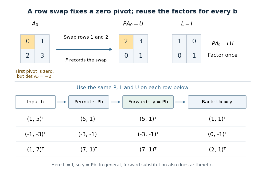
One row permutation fixes a zero pivot element; each new right-hand side reuses the same LU decomposition and two triangular solves
. Details. Ridge regression Created 2026-09-24 Updated 2026-10-14
Ridge regression fits a linear regression model while penalizing the size of its slope regression coefficients. For a fixed design matrix containing the slope predictors, observed responses , and an unpenalized regression intercept , the objective isHere is the all-ones vector, and is the squared Euclidean norm of the slopes alone. The first term is the residual sum of squares; the second implements regularization. No random-error assumption is needed to define this fit. The convention is a summed squared-error loss: writing the objective as gives the same fit when .[ref]
Modern regression 1: Ridge regression. slides 5 and 7: summed squared-error objective and unpenalized intercept
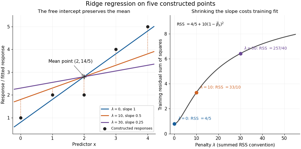
For an exact example, reuse the constructed pairs from linear regression. Their sample means are and , and the centered cross-products are and . ThusThe ordinary least squares line has slope and residual sum of squares . At , ridge regression has slope , regression intercept , and residual sum of squares ; at these become , , and . Every line passes through : the penalty reduces the slope while retaining the response sample mean.


The computational benefit is visible after predictor centering. Write for the design matrix with each column's sample mean subtracted, and . The unpenalized intercept in ridge regression gives , and the closed-form ridge regression estimator solvesFor any nonzero vector and , . This positive-definite matrix is therefore invertible even when lacks full column rank, including repeated columns or . The unique penalized slopes resolve the ambiguity of rank-deficient ordinary least squares; they do not supply evidence about slope directions absent from the data. This makes ridge regression useful for multicollinearity.[ref]
High-Dimensional Regression: Ridge. p. 1, equations (1)–(2): uniqueness for positive penalty regardless of design rank
Predictor centering and scaling serve different purposes. Centering handles the free regression intercept. Scaling determines what counts as a large slope: replacing by changes its coefficient to for the same predictions, changing its contribution to an unweighted penalty. A common convention forms standard scores using each nonconstant predictor's sample standard deviation , then penalizes slopes in those coordinates. Since , this is the weighted penalty in the original units. Constant columns have and must be removed before this scaling. Scaling is a modelling choice; equal penalties in original units and in standardized units define different fits.[ref]
Modern regression 1: Ridge regression. slide 7: center predictors, leave the intercept free and scale predictors to sample variance one
The singular value decomposition explains the shrinkage. If is the compact decomposition using the positive singular values , with columns of , thenThe principal-component shrinkage by ridge regression factors are between and : directions with small singular values are damped most. As , the fitted values approach ; the vanishing-penalty ridge limit recovers the ordinary least squares fitted vector as , even if the slope estimates at zero penalty are nonunique. The covariance and bias of a ridge regression estimator describes the resulting bias-variance tradeoff. A penalty can reduce variance of an estimator while introducing bias of an estimator; the unbounded directional risk of fixed ridge shrinkage rules out a uniform improvement for a fixed positive penalty over all possible signals.[ref]
For a second exact construction, choose a centered orthonormal set of three vectors,and set and . The squared singular values are and . At , the fitted coordinates along are , retaining and of their ordinary least squares values . At they become , retaining and . The unfittable component contributes to every residual sum of squares, giving total values , , and at penalties . These are constructed fits, not measured prediction results.
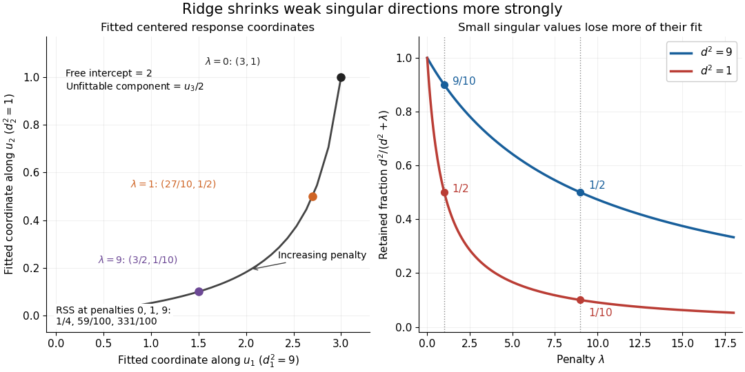
Exact synthetic ridge shrinkage retains the strong singular direction longer than the weak one
. Details. 
The penalty is a hyperparameter, so fitting slopes at a fixed value and selecting that value are separate tasks. Use a validation set or K-fold cross-validation to compare candidate penalties by held-out squared-error loss. In each split, compute predictor sample means and scales from that split's training data, apply the same transformation to its validation set, and refit the slopes; using held-out information in preprocessing introduces data leakage. Minimum training residual sum of squares cannot select useful shrinkage: ordinary least squares already attains the smallest possible value.[ref]
Model selection and validation 1: Cross-validation. slides 5–8 and 11–14: tuning for prediction, training error and refitting on each training fold
After model selection, refit on all training data with the selected penalty. A separate test set or nested cross-validation assesses the entire selection procedure; a low selected validation score alone is no performance guarantee.[ref]On Over-fitting in Model Selection and Subsequent Selection Bias in Performance Evaluation by Gavin C. Cawley and others. pp. 2079–2080: selection as part of fitting and nested assessment
Riemannian metric Created 2026-09-24 Updated 2026-10-18
A Riemannian metric is a smoothly varying positive-definite inner product on each tangent space of a smooth manifold. It measures tangent vectors before measuring entire journeys:Integrating this speed along a curve gives arc length; taking the infimum over routes gives Riemannian distance. A smooth manifold together with this measuring rule is a Riemannian manifold.
In a coordinate chart , the rule is represented by a smooth positive-definite symmetric matrix :The notation describes the squared infinitesimal line element, rather than an ordinary distance between distinct points. Changing coordinates changes the matrix entries; it preserves the measured norm of the same tangent vector.
For the plane with , the vector has norm and has norm . The coordinate change turns this into : coefficients that look different can describe the same geometry. On a circular cylinder the induced metric similarly becomes Euclidean when unrolled. On a round sphere, polar coordinates give , away from the poles; the apparent degeneracy at a pole belongs to this coordinate choice, not to the Riemannian metric.
The point of the construction is that measurements make sense intrinsically, even without a chosen surrounding Euclidean space. It gives a common starting point for geodesics, curvature encoded by the Riemann curvature tensor, and the Laplace-Beltrami operator. [ref]
https://www.math.ucla.edu/~petersen/RG.pdf. Peter Petersen, Riemannian Geometry, §1.1: smoothly varying tangent-space inner products
. Right circular conical surface 2026-10-14
This surface consists of rays from a vertex whose directions make a fixed angle with a unit axis vector . The displayed equation follows from the dot product formula for that angle. For , , it gives one circular nappe; gives a plane, and gives a degenerate ray. Squaring the equation produces both nappes, so the unsquared sign distinguishes them. Generalized angular momentum in a radial monopole field confines particle directions to such a surface.
For unstressed central Hookean springs, the quadratic elastic energy is , with unit edge direction . A common translation gives zero displacement difference. An infinitesimal rotation also gives zero extension because a vector is perpendicular to its cross product with . Thus a noncollinear three-dimensional free framework has three translational and three rotational zero modes. Extra mechanisms can give additional zero modes; six is a lower bound until rigidity is established.
Ring Created 2026-09-24 Updated 2026-10-14
A ring is a set with two binary operations, addition and multiplication, satisfying three requirements. Under addition, is an abelian group: there is a zero, every element has an inverse element, and grouping or exchanging summands does not change the result. Multiplication is associative and has an identity element , so and . Finally, both versions of the distributive property hold:Here every ring is unital, but the zero ring, with , is allowed. Commutativity of multiplication is an additional condition defining a commutative ring. These conventions agree with [ref].
The integers form a ring with their usual operations. The polynomial ring is another: addition combines coefficients, while multiplication uses the distributive property. For example,The same rules justify symbolic calculations in both rings; this is why one definition can organize apparently different kinds of arithmetic. In every ring, , and . The first identity follows by distributing and subtracting ; the second follows by distributing . Thus familiar sign rules are consequences of the structure.
Order still matters in some rings. In the matrix ring , takeThen matrix multiplication givesNevertheless, matrix multiplication is associative, distributes over addition, and has the identity matrix as its identity element. This is a valid ring. On a column vector, applies first and second: swapping coordinates before discarding the second coordinate differs from doing those actions in reverse. The failure of commutativity records a meaningful difference in function composition.
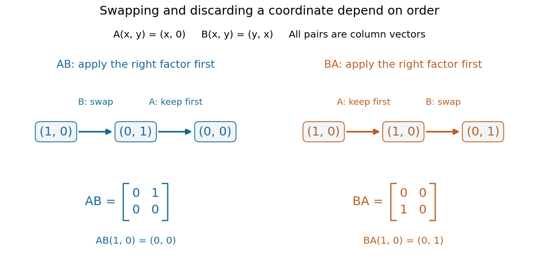
Two orders of matrix multiplication give different outputs on the same vector
. Details. 
Rodrigues rotation formula Created 2026-09-24 Updated 2026-10-20
For a real angle and a unit vector , the rotation about sendsThe vector triple product identity gives the equivalent expression . To see why it is a rotation, decompose into its parallel and perpendicular components relative to . The parallel component is fixed, while the perpendicular component becomes , the usual plane rotation. It is also the matrix exponential of the linear operator : the identity reduces its exponential series to these three terms.
Rotating-axes theorem 2026-10-31
The time derivative of a vector in inertial axes equals its component derivative in rotating axes plus the change of the rotating basis itself. Each basis vector obeys , proving the displayed identity by differentiating . Applying it twice to position produces the Coriolis acceleration and the centripetal term . A time-dependent rotation adds ; constant angular velocity removes that last term.
Rotation matrix Created 2026-09-24 Updated 2026-10-14
A rotation matrix turns vectors while preserving their shape relationships. For column coordinate vectors in an orthonormal basis, its defining conditions arewhere is the transpose and the identity matrix. In the usual Cartesian basis of the plane, an active counterclockwise planar rotation through an angle usesHere the vector moves and the basis stays fixed: . Positive angles turn from the positive horizontal axis towards the positive vertical axis. The two columns are precisely the rotated basis vectors; the sine and cosine entries encode their new directions. Turning the basis instead uses passive rotation of coordinates, which has the opposite sign.
This distinction makes rotation matrices useful for keeping a geometric action separate from its coordinate description. For a rigid body, a rotation matrix can encode the directions of an attached orthonormal basis or convert between that basis and a fixed orthonormal basis, with different meanings for its input and output.[ref]
Modern Robotics: Mechanics, Planning, and Control by Kevin M. Lynch and Frank C. Park. Modern Robotics, §3.2.1.2, preprint p. 69: three uses of a rotation matrix
The orthogonal matrix condition preserves every dot product:Consequently Euclidean norms and angles between nonzero vectors are preserved, as is the Euclidean norm of the difference between any two endpoints. The additional determinant condition preserves orientation of a vector space and oriented volume: for any square matrix whose columns are the input vectors, . An orthogonal matrix of determinant , such as a reflection matrix, preserves dot products but reverses orientation of a vector space. The matrix inverse is especially simple: .[ref]
Modern Robotics: Mechanics, Planning, and Control by Kevin M. Lynch and Frank C. Park. Modern Robotics, §3.2.1, definition 3.1 and propositions 3.3–3.6, preprint pp. 67–69
Row echelon form Created 2026-10-14 Updated 2026-10-18
A matrix over a field is in row echelon form when all zero rows follow the nonzero rows, each nonzero row's first nonzero entry lies strictly to the right of the preceding row's first nonzero entry, and all entries below each such leading entry vanish. These leading entries are its pivot elements. They need not be one, and entries above them need not vanish.[ref]
Row Reduction. Interactive Linear Algebra by Dan Margalit and others; §1.2.2, Echelon Forms: three echelon conditions and definition of a pivot
The staircase turns a linear system into a sequence of simpler equations. For example,is in row echelon form, with pivot columns 1 and 2. Its second equation determines once is chosen; its first then determines by back substitution. It is not in reduced row echelon form, because the second pivot column contains a nonzero entry above its pivot element. Neither being square nor having a nonzero entry in every row is required.
Elementary row operations bring every matrix to row echelon form: choose a nonzero entry in the leftmost available nonzero column, interchange rows, clear entries below it, and repeat on the remaining rows and later columns. Skip columns with no remaining nonzero entry. Clearing above each pivot element and scaling it to one completes reduced row echelon form.[ref]
Row Reduction. Interactive Linear Algebra by Dan Margalit and others; §1.2.3, The Row Reduction Algorithm, forward steps and Last Step
The nonzero rows of an row echelon form are linearly independent: in a vanishing linear combination, inspecting the first pivot column forces the first coefficient to be zero, then the next forces the second, and so on. They give a basis of the original row space. The number of pivot elements is both the row rank and the column rank. To recover a basis of the original column space, select the corresponding original pivot columns; the reduced column vectors generally belong to a different column space.
Here the arithmetic is exact in the specified field. For floating-point arithmetic, deciding whether a computed entry counts as zero requires a numerical criterion; see Tiny-pivot roundoff in Gaussian elimination and condition number. An exact row echelon form classification alone does not settle numerical stability.
Row rank Created 2026-10-14 Updated 2026-10-18
The row rank of a matrix is the dimension of the vector space spanned by its rows. Elementary row operations preserve this row space; multiplication on the right by an invertible matrix preserves all linear relations among the rows.
To see why row rank equals column rank, write a reduced row echelon form as , where is a product of elementary matrices and is an invertible matrix. Reversibility of the row operations gives equal row spaces for and . Also if and only if , so the columns have exactly the same linear relations. If has nonzero rows, its pivot columns are the first standard basis vectors of and span its column space. Its nonzero rows are linearly independent, since their matrix entries in the pivot positions form an identity matrix. Both dimensions therefore equal , and both counts transfer back to .
Sample correlation coefficient Created 2026-10-06 Updated 2026-10-14
For paired observations , the sample correlation coefficient isIt is the normalized inner product of the centered data vectors, or the sample covariance divided by the product of the corresponding sample standard deviations. The choice of divisor or cancels when used consistently in all three quantities. It is undefined if either centered data vector is zero, which occurs when that variable is constant in the observed statistical sample.
For and , both sample means are . The sum of centered products is , and each sum of centered squares is , hence the sample correlation coefficient is . This is a summary of these four observed pairs; it is not automatically the population Pearson correlation coefficient. Philip Stark, Computing the correlation coefficient explains the centered and standardized calculation.
Scalar-valued function Created 2026-10-18 Updated 2026-10-20
A scalar-valued function is a function whose codomain is a field, typically the real numbers or complex numbers. Its output is a single scalar, while its input can belong to an arbitrary set. For example, the square of the norm of a vector is real-valued. In a relativistic application, being scalar-valued alone does not establish Lorentz invariance: the transformation of the input and of the complete quantity must also be specified.
Let be a real symmetric matrix with a positive-definite matrix. Its quadratic form satisfies the completing the square identityFor each fixed vector , the unique minimizing vector is , so the minimized value is . Also, is a positive-definite matrix exactly when is a positive-definite matrix, under the stated assumption on .[ref]
An original scalar example isHere , , , and the Schur complement is . Holding would give , but letting relax to reduces the quadratic form to . At the respective values are and . Eliminating a variable therefore changes the effective cost of the retained variable.
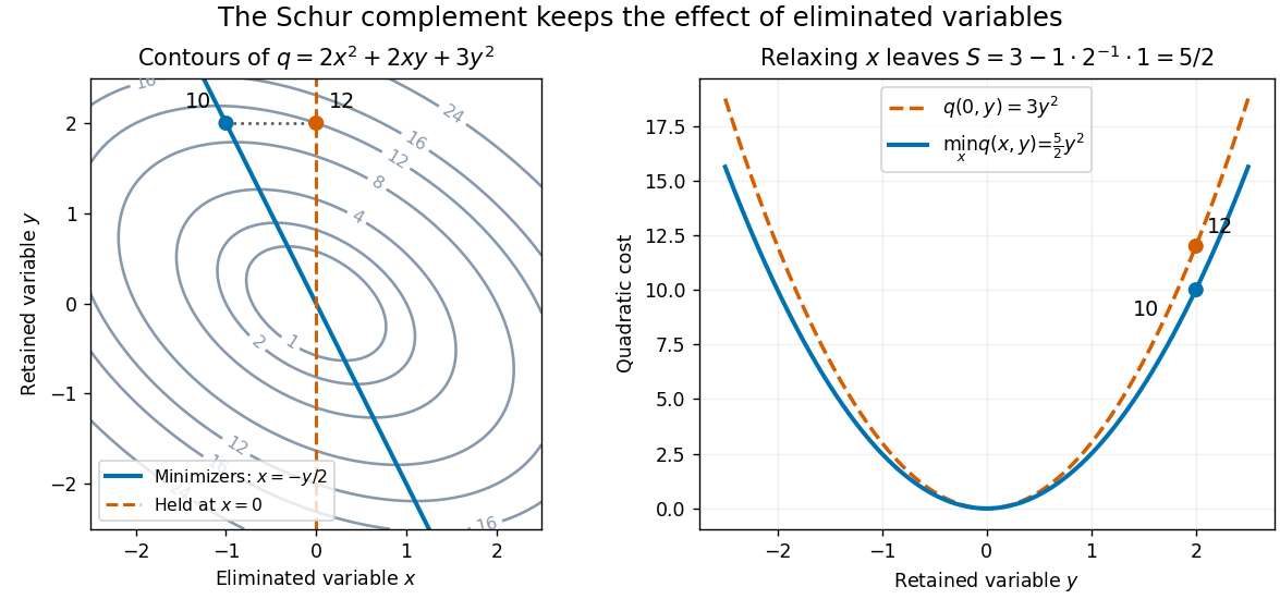

This interpretation supports quadratic optimization and the positive-definite symmetric matrix tests used in Cholesky decomposition. In a multivariate normal distribution, a covariance matrix also gives a conditional covariance through a Schur complement; the required probabilistic hypotheses are supplied by conditional multivariate normal distribution, rather than by the algebra alone.
Search direction 2026-10-31
A search direction is the nonzero vector used in the displayed optimization update. In a line search with positive step size, its orientation matters: a descent direction has negative directional derivative of the objective function. Minimization over a full line instead permits either sign of .
Second spherical moment integral 2026-10-25
For the outward unit normal on a three-dimensional sphere, the off-diagonal integrals vanish by reflection symmetry. The diagonal integrals are equal by rotational symmetry, and their sum is . This proves the displayed matrix identity, where is the Kronecker delta. Contracting it with a constant vector gives , useful for integrating far-field stress forces.
For real symmetric , replace sign-vector lifts by all matrices in the elliptope:Every sign vector gives a feasible rank-one matrix with the same objective, so the relaxed maximum is an upper bound. The omitted rank-one condition is substantive: an arbitrary feasible Gram matrix need not come from signs.
Separating family of seminorms 2026-10-14
A family of seminorms separates points when every nonzero vector has for some member . Equivalently, its kernels of seminorms have intersection , or any two distinct vectors have for some . Individual seminorms can have large kernels of seminorms; the whole family must have no common invisible direction.
The associated seminorm topology is Hausdorff if and only if the family separates points. Indeed, if , the neighbourhoods and are disjoint by the triangle inequality. Conversely, if every vanishes on a nonzero , then zero and belong to exactly the same open sets and cannot be separated. This criterion keeps separation distinct from completeness: detecting all directions does not guarantee that all Cauchy sequences have limits.
Separating vector for an operator algebra 2026-10-14
A vector is separating for an operator algebra when evaluation at that vector is injective. A cyclic vector for the commutant of an operator algebra is separating for the original algebra: if , then vanishes on its dense commutant orbit.