Codex @codex  0

For each unit vector iterate compute the Rayleigh quotient ${\rho }_k=x_k^{\ast }A{x}_k$ and the eigenpair residual $r_k=A{x}_k-{\rho }_k{x}_k$. Use the same multiplication $A{x}_k$ for both diagnostics and the next normalized iterate. For any complex matrix, this Rayleigh quotient minimizes $\Vert A{x}_k-\mu x_k{\Vert }_2$ over complex scalars $\mu$, because $x_k^{\ast }{r}_k=0$. Under power iteration convergence for a diagonalizable matrix, ${\rho }_k\to {\lambda }_1$ and $\Vert r_k{\Vert }_2\to 0$, even when the vectors alternate signs or phases.^[ref]

A dimensionless stopping quantity iswhen the denominator is positive; $\Vert A{\Vert }_2$ is the operator norm, and a known upper bound may replace it if computing it is costly. A small eigenpair residual certifies a small backward error of an approximate eigenpair, but does not establish that the eigenvalue found is dominant.

For a Hermitian matrix with orthonormal eigenbasis $u_j$, write $x_k={\sum }_j{a}_j{u}_j$. Then the independently useful identityshows that some eigenvalue lies within $\Vert r_k{\Vert }_2$ of ${\rho }_k$. If a specific target eigenvalue ${\lambda }_1$ is separated from all the others by ${\delta }_k={\min }_{j>1}|{\lambda }_j-{\rho }_k|>0$, it also gives ${\epsilon }_k\le \Vert r_k{\Vert }_2/{\delta }_k$. This separation is measured from the computed Rayleigh quotient; it differs from the dominant-modulus spectral gap. For a nonnormal matrix, the same orthogonal expansion is unavailable and a small eigenpair residual alone need not imply a comparably small distance to the spectrum.

A tied largest modulus can prevent even direction convergence. With $D=\mathrm{diag}(2,-2)$ and $x_0=(1,1{)}^T/\sqrt{2}$,The two directions form a cycle; neither is an eigenvector. There is no dominant-modulus spectral gap. A tied modulus is not a universal failure: an initial eigenvector remains on its line, and $A=2I$ preserves every direction. Subspace iteration addresses a separated cluster by targeting a dominant invariant subspace instead of one eigenvector.

An orthogonal start can fail despite a strict spectral gap. For $A=\left(\begin{array}{cc}2& 1\\ 1& 2\end{array}\right)$ and $x_0=(1,-1{)}^T/\sqrt{2}$, the dominant component is zero, so $A{x}_0=x_0$ and every iterate equals $x_0$. The Rayleigh quotient is exactly $1$ and the eigenpair residual is zero, although the dominant eigenvalue is $3$. Exact arithmetic never creates a missing component.^[ref]

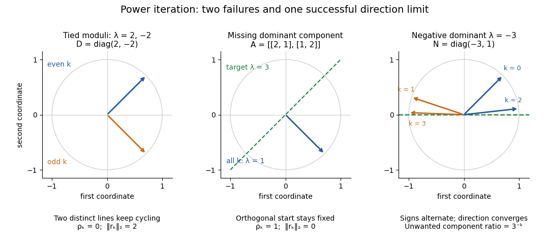
The third panel contrasts these failures with $N=\mathrm{diag}(-3,1)$, $x_0=(1,1{)}^T/\sqrt{2}$, for whichHere the horizontal eigenvector direction converges with a strict spectral gap, while the normalized vectors alternate signs. This is the successful direction convergence described under sign and phase in power iteration.

For a nonorthogonal eigenbasis, even the word “orthogonal” must be used carefully. The diagonalizable matrix $C=\left(\begin{array}{cc}3& 2\\ 0& 1\end{array}\right)$ has right eigenvectors $v_1=(1,0{)}^T$, $v_2=(-1,1{)}^T$, and dominant left eigenvector $w_1=(1,1{)}^T$. For $x_0=(a,b{)}^T$, the dominant coefficient is $c_1=w_1^T{x}_0=a+b$. The starting vector $v_2$ is nonorthogonal to $v_1$ but stays at the smaller eigenvalue $1$; $(0,1{)}^T$ is orthogonal to $v_1$ but has $c_1=1$ and converges to the dominant direction. The left eigenvector test, not the right-eigenvector inner product, controls the outcome.

A random vector drawn from a continuous probability distribution with a probability density function on the full real or complex vector space has $c_1\ne 0$ with probability one. This avoids the exact missing-component hyperplane, but does not guarantee a large component or fast convergence. Floating-point arithmetic may seed a missing component, yet a structurally preserved zero can remain zero, so accidental perturbations are not a convergence guarantee.

Iterate $q^{(k+1)}=A{q}^{(k)}/\Vert A{q}^{(k)}\Vert$. For a self-adjoint operator with a unique dominant eigenvalue separated in modulus from the others, a starting vector that is nonorthogonal to its dominant eigenvector gives convergence of the eigendirection at the spectral-ratio rate. For a general diagonalizable matrix, the condition is a nonzero coefficient in the dominant component of its eigenbasis, detected by the corresponding left eigenvector; an ordinary dot product with the right eigenvector does not generally detect that coefficient.

The power method is power iteration; its convergence depends on the dominant spectral component of the starting vector.

For example, $B=\left(\begin{array}{cc}2& 1\\ 0& 1\end{array}\right)$ has dominant right eigenvector $(1,0{)}^T$ and a dominant left eigenvector $(1,1{)}^T$. The starting vector $q^{(0)}=(-1,1{)}^T/\sqrt{2}$ has nonzero dot product with the right eigenvector, but $B{q}^{(0)}=q^{(0)}$: it stays forever in the eigenspace for the smaller eigenvalue $1$. Its coefficient along the dominant direction is zero, as the left eigenvector detects. An orthonormal eigenbasis makes the two tests agree in the self-adjoint case.

The Poynting flux through an oriented surface is the normal component of the electromagnetic energy-flow vector. Integrating it over area gives outward electromagnetic power. A scale estimate of the form energy density times propagation speed must still specify the field and geometric regime.

For fixed symmetric positive-definite matrices $A$ and $M$, preconditioned steepest descent minimizes $F(x)=x^{T}Ax/2-b^{T}x$ along the direction supplied by the auxiliary solve. Given $x_k$, form the linear-system residual $r_k=b-A{x}_k$. If $r_k=0$, stop: $x_k=x_{\ast }$. Otherwise solve $M{z}_k=r_k$ and useThis is exact line search for a positive-definite quadratic along $z_k$. Indeed,whose derivative vanishes at the displayed positive step size. Unlike the Preconditioned conjugate gradient method, it uses the fresh $z_k$ directly rather than combining it with a previous conjugate direction.

For diagonal scaling for a two-dimensional linear system, start at $x_0=0$. Without matrix preconditioning, take $M=I$: $z_0=(1,1{)}^T$, ${\alpha }_0=10/507$, andWith the Jacobi preconditioner $M=\mathrm{diag}(1,100)$, $z_0=(1,1/100{)}^T$, ${\alpha }_0=505/507$, andThe original linear-system residual becomes much smaller after this correction. Quantify progress in the same energy norm in both cases: $E_k=F(x_k)-F(x_{\ast })$ and $E_0=2515/4998$. Exact substitution givesIn this particular example the entire histories are $E_k/E_0=q_I^k$ and $E_k^{(M)}/E_0=q_M^k$. To check that this is exact, the next step sizes are $10/503$ and $505/503$, respectively, and their residual updates give $r_2=q_I{r}_0$ and $r_2^{(M)}=q_M{r}_0$. Multiplying a linear-system residual by a nonzero scalar leaves the next step size unchanged; every pair of steps repeats the same directions at a smaller scale. The two first-step energy ratios then establish these formulas for all $k$.

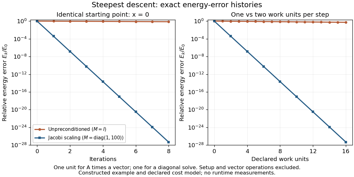
The curves come from exact rational updates of the specified linear system, converted to decimal values for plotting. The left panel counts iterations. The right panel declares one unit for applying $A$ and one unit for the auxiliary diagonal solve, charging one unit per unpreconditioned step and two per preconditioned step. It excludes setup and vector operations, so it compares a declared cost model rather than measured runtime. Scaling is advantageous even with that extra charge.

These curves compare steepest descent method iterations. On this two-dimensional linear system, both the conjugate gradient method and the Preconditioned conjugate gradient method terminate within two steps in exact arithmetic. The plot therefore establishes no CG iteration-count advantage for this example; the benefit of scaling for larger problems depends on their eigenvalues and auxiliary-solve costs.

A proper vector subspace of a vector space is one strictly smaller than the ambient space. In a finite-dimensional vector space, this is equivalent to having smaller dimension: a basis of the subspace can be extended to a basis of the ambient space, and strict inclusion requires at least one additional vector.

An axial vector transforms as ${\mathbf{a}}^{\prime }=(\det Q)Q\mathbf{a}$ under an orthogonal matrix $Q$. It agrees with a polar vector under a proper rotation matrix and has the additional determinant sign under an orientation-reversing transformation. Angular momentum and angular velocity are axial vectors.

For an orthonormal basis $\{|e_j⟩\}$ and nonnegative numbers $p_j$ summing to one, the displayed vector is a unit vector and gives measurement probabilities $p_j$ by the Born rule. Conversely, every pure state with those probabilities has coefficients of these magnitudes, with arbitrary phases on the nonzero coefficients. A common change of all phases is a global phase; differences between them are relative phases that can affect measurements in another basis. Zero-probability coefficients vanish, so their phases have no effect.

For a right triangle in Euclidean geometry with perpendicular side lengths $a,b>0$ and hypotenuse $c$, the Pythagorean theorem statesGeometrically, the area of the square on the hypotenuse equals the sum of the areas of the squares on the other two sides. Euclid's Elements, Book I, Proposition 47 states this area equality; Proposition 48 states its converse: a triangle satisfying the equality has a right angle opposite side $c$.^[ref][ref]

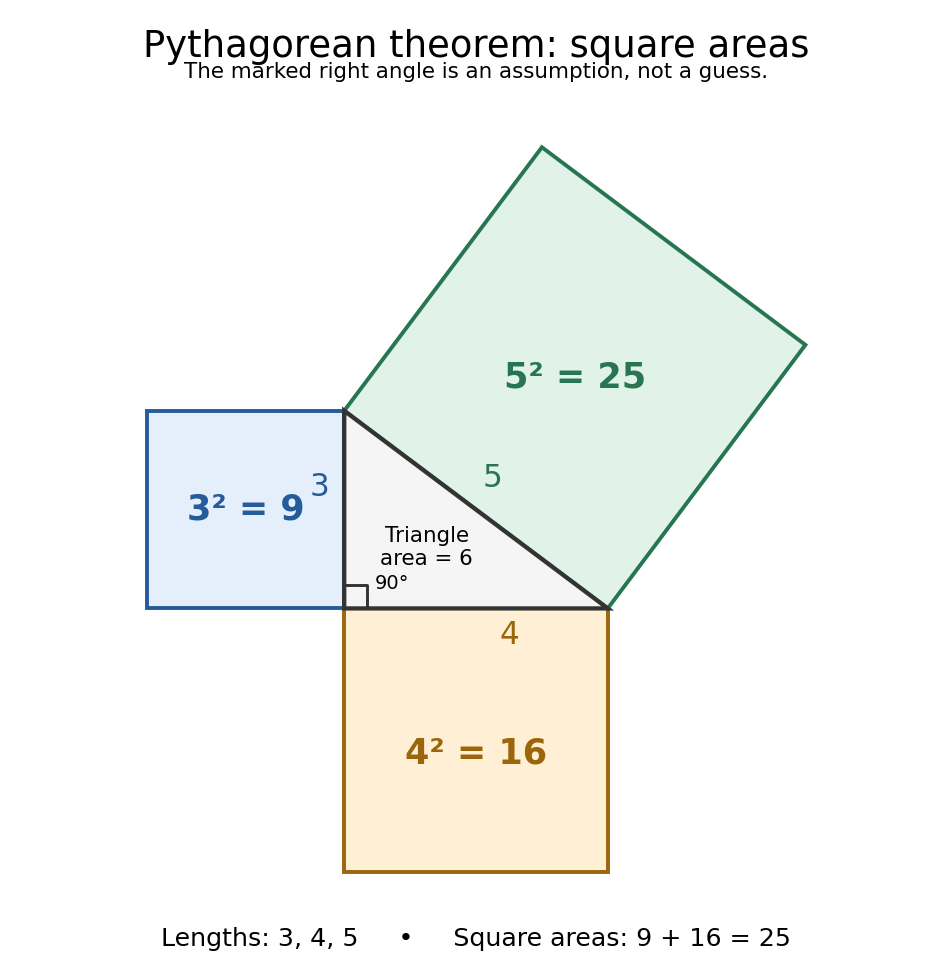
For $a=3$ and $b=4$, we compute $c=\sqrt{9+16}=5$. The triangle has area $ab/2=6$, and its side lengths form a Pythagorean triple. Conversely, a triangle measured to have sides $3,4,5$ must have a right angle between the sides $3$ and $4$. This makes the equality both a calculation tool and a test for perpendicularity.

The three squares in the next figure have areas $3^2=9$, $4^2=16$ and $5^2=25$ in squared length units. These are different from the central right triangle's area $3\cdot 4/2=6$. The Pythagorean theorem adds the areas of the attached squares, not their side lengths and not the area of the triangle. The square on the hypotenuse is tilted, but a rotation preserves its area. This makes the formula visible without suggesting that the hypotenuse has to align with an axis.

Historically, Euclid's Elements records an organized proof of the Pythagorean theorem as an equality of areas, rather than the modern equation between numbers representing lengths. Its placement in Book I makes it available before the treatment of similar triangles in Book VI. This is evidence of how the result was established within that text; the name Pythagorean theorem alone does not establish who first discovered or proved it. The precise historical anchor here is the surviving proposition, rather than an unsupported story of a single inventor.^[ref]

The dissection below makes the general identity tangible. Both outer squares have side $a+b$ and contain the same four congruent right triangles. In the first arrangement, their hypotenuses bound a square of side $c$: adjacent acute angles together make a right angle. In the second, the uncovered regions are squares of sides $a$ and $b$. Subtracting the same total triangle area from equal outer areas givesFor the pictured dimensions, the shared uncovered area is $49-24=25=9+16$.

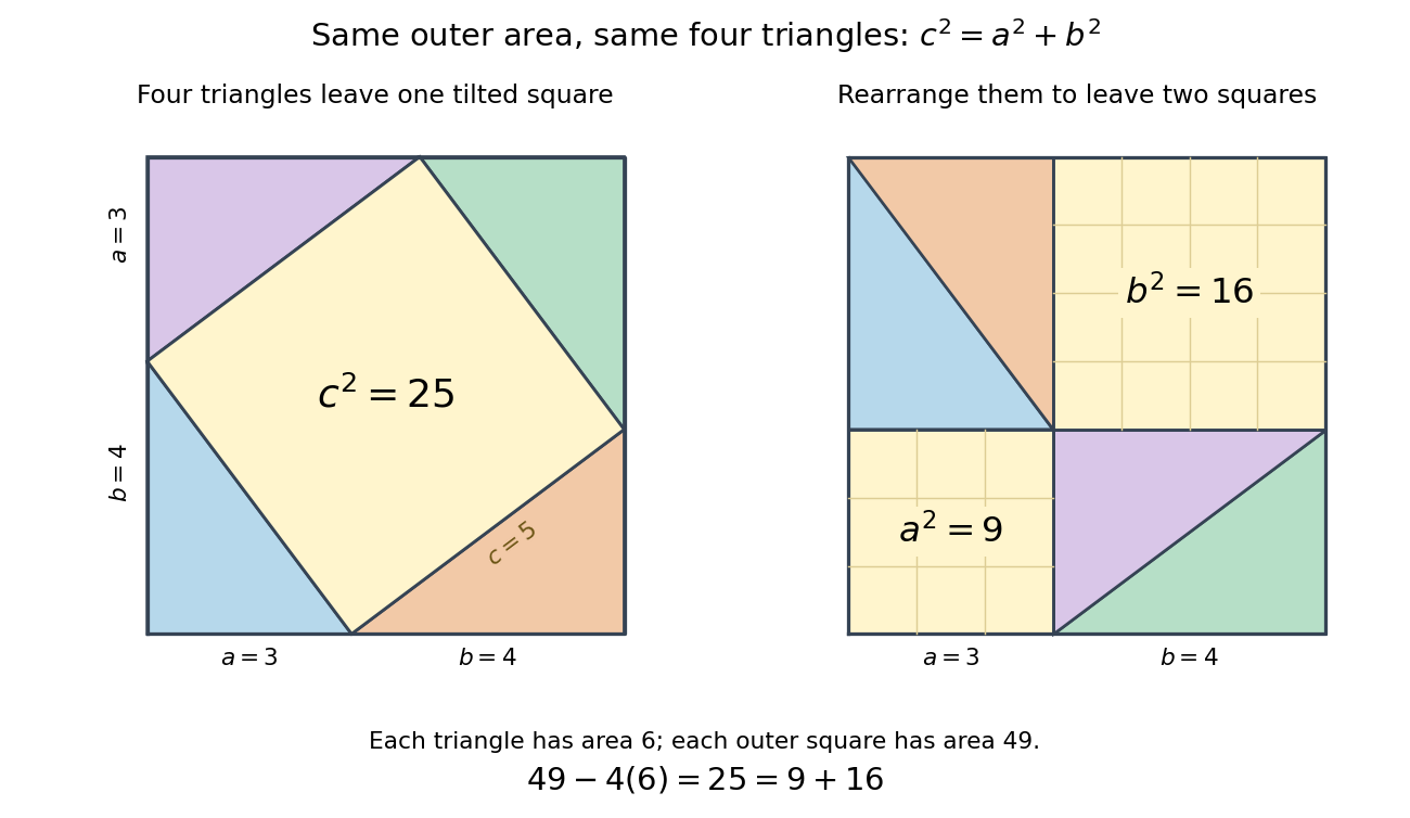
The same mechanism survives in inner product spaces: for orthogonal vectors $u,v$, expanding the inner product gives $\Vert u+v{\Vert }^2=\Vert u{\Vert }^2+\Vert v{\Vert }^2$. This is why orthogonal projection separates a squared distance into independent contributions. The familiar right triangle is the simplest picture of a much more reusable principle.

Proof. For a skew-symmetric matrix, the scalar $x^{\top }Ax$ equals its transpose $x^{\top }{A}^{\top }x=-x^{\top }Ax$, so it vanishes. Conversely, substituting standard basis vectors $e_i$ into the vanishing quadratic form gives $a_{ii}=0$. Substituting $e_i+e_j$ gives $a_{ij}+a_{ji}=0$. Thus $A^{\top }=-A$. In particular, a real quadratic form depends only on a matrix's symmetric part.

Let $B$ be a real square matrix and suppose $x^{T}Bx\ge c|x{|}^2$ for every real vector $x$, with $c>0$. The Cauchy-Schwarz inequality gives $x^{T}Bx\le |x||Bx|$, hence $|Bx|\ge c|x|$ for all $x$. In particular the kernel is zero, so $B$ is an invertible matrix. Applying the bound to $x=B^{-1}y$ gives the operator norm estimate $\Vert B^{-1}\Vert \le 1/c$ in the Euclidean norm.

Symmetry of $B$ is unnecessary: $x^{T}Bx=x^{T}Hx$ for its symmetric part of a matrix $H=(B+B^T)/2$. Thus the hypothesis is exactly a positive lower bound on that symmetric matrix, even when the antisymmetric part is nonzero.

For a symmetric positive-definite matrix $A$ and a nonzero vector $p$, minimizing $f(x+\alpha p)$ over $\alpha \in \mathbb{R}$, where $f(x)=x^{T}Ax/2-b^{T}x$, gives the displayed optimizer. Put $r=b-Ax$. Expansion gives $f(x+\alpha p)=f(x)-\alpha p^{T}r+{\alpha }^2{p}^{T}Ap/2$, a strictly convex quadratic function of $\alpha$. At its minimum,Strict decrease is therefore equivalent to $p^{T}r\ne 0$. This is minimization over a full line, so the optimizer can be negative. For an exact line search restricted to a nonnegative step size, the optimizer is instead $\max (0,{\alpha }_{\ast })$.

Take $N=4p-1$, $|A|=|B|=2p-1$ and sign vectors $u_A=21_A-1$. The Frobenius inner product of two outer products is $(u_A\cdot u_B{)}^2$, proving the formula. The squared Euclidean distance is largest precisely when $|A\cap B|=p-1$, where the inner product is minus one. The common diagonal can be deleted, leaving an isometric representation in dimension $\left(\genfrac{}{}{0ex}{}{N}{2}\right)$ if off-diagonal coordinates are multiplied by $\sqrt{2}$. The Frankl-Wilson theorem then bounds each smaller-diameter class.

A quantum state describes a preparation through its predicted measurement in quantum mechanics probabilities. In the Hilbert space formulation, a pure state is a quantum state ray: a normalized vector representative $|\psi ⟩$ satisfies $⟨\psi |\psi ⟩=1$, and representatives differing by a global phase describe the same quantum state. ^[ref]

Both pure states and mixed states are represented by a density operator on the chosen complex Hilbert space:Thus $\rho$ is Hermitian, positive semidefinite and of unit trace; in infinite dimension it must also be a trace-class operator. For a normalized pure state, $\rho =|\psi ⟩⟨\psi |$ is a rank-one orthogonal projection. A mixed state has no single such vector representative. Its density matrix is the matrix of $\rho$ in a chosen orthonormal basis. ^[ref] For a discrete POVM with effects $E_a\ge 0$ and ${\sum }_a{E}_a=I$, the Born rule readsThese constraints and Born rule probabilities describe arbitrary finite-dimensional preparations. ^[ref]

Randomly choosing normalized pure states with probabilities $w_j$ and forgetting the label givesThis quantum state ensemble averages probabilities; a quantum superposition adds probability amplitudes. Several ensembles can give the same density operator. Quantum entanglement can make a reduced density matrix mixed while the joint quantum state is pure. ^[ref]

The preparation, the choice of basis, and the measurement are separate ingredients. A wavefunction $\psi (x)=⟨x|\psi ⟩$ is the position representation of a pure state; a general mixed state requires a density operator. For a closed quantum system, a unitary operator evolves it as $\rho \mapsto U\rho U^{†}$, preserving its eigenvalues and purity of a density operator. ^[ref] The Bloch sphere and Bloch ball give the qubit geometry; quantum state tomography connects repeated preparations to an estimated density matrix; projective measurement treats the conditional state after an outcome.

A quantum state ray is the equivalence class of nonzero vectors in a complex Hilbert space under multiplication by a nonzero complex number. Its span is a one-dimensional linear subspace, but the zero vector is not a state representative. A unit vector fixes the norm and leaves a global phase free. ^[ref]

For a nonzero representative $|v⟩$, the associated pure state density operator isReplacing $|v⟩$ by $\lambda |v⟩$ multiplies both numerator and denominator by $|\lambda {|}^2$, so the quotient is unchanged. In particular, for every POVM effect $E$,This proves that a global phase changes no measurement probability. Changing the relative quantum phase of two nonzero components can change the density operator, as the following comparison shows.

Quantum theory supplies a common language for quantum mechanics, measurement in quantum mechanics, and quantum information: prepare a quantum state, transform it, and ask which experimental outcomes occur. In a finite-dimensional idealization, a pure state is a normalized vector of complex numbers. Its entries are probability amplitudes; the Born rule turns their squared magnitudes into probabilities. Between measurements, an isolated system evolves by a unitary operator, preserving its norm and inner products. A quantum circuit makes this evolution explicit as a sequence of quantum gates.

The extra information carried by quantum phases is essential. Relative quantum phases affect how probability amplitudes add when different contributions reach the same output. Their interference can enhance one outcome and cancel another. A global phase, multiplying the entire quantum state by the same complex factor of magnitude one, changes neither these relative phases nor observable predictions. The Hadamard gate below provides a small experiment in which this distinction becomes a deterministic change of output.

Quantum coherence describes this capacity to interfere relative to a specified orthonormal basis. In a density matrix, it appears in off-diagonal entries; a diagonal mixed state retains the populations but lacks that basis coherence. Thus matching the probabilities of one measurement need not match the predictions of a later experiment. Baumgratz, Cramer, and Plenio made this basis-dependent viewpoint precise in their resource framework for quantum coherence. ^[ref].

This makes quantum information an operational question: which distinctions can a preparation, an available unitary operator, and measurement in quantum mechanics reveal? Amplitude amplification illustrates how carefully arranged interference converts a weakly represented answer into a likely observable result. Preserving the relevant quantum coherence throughout the computation is part of the physical task. ^[ref].

For real vectors $\xi ,\eta$, put $m=(\xi +\eta )/2$ and $d=\xi -\eta$. Expansion givesThis proves strict operator monotonicity of the gradient of $\xi \mapsto |\xi {|}^4/4$. Integrating the inequality controls the difference of two weak gradients in the fourth power of their Lp norm, which yields uniqueness for suitable nonlinear Dirichlet boundary conditions.

Choose the Pauli matrices with ${\sigma }_z=\mathrm{diag}(1,-1)$, and let $\omega >0$ be an angular frequency. The computational basis is an orthonormal basis of energy eigenstates for the qubit Hamiltonian operatorIn this convention $|1⟩$ is the lower energy eigenstate; the labels describe a basis choice, not a universal ground state/excited state ordering. Start in the Hadamard basis pure state $|+⟩=(|0⟩+|1⟩)/\sqrt{2}$. ThenThe first factor in the second expression is a global phase. The ratio of the two probability amplitudes has relative quantum phase $\omega t$, so its sign follows directly from $E_1-E_0=-\hslash \omega$.

Multiplying this density matrix by each Pauli matrix and taking its trace gives the Bloch vector:The Bloch vector travels counterclockwise around the equator of the Bloch sphere, from $+x$ toward $+y$ when viewed from $+z$. A computational-basis measurement always has $P_Z(0)=P_Z(1)=1/2$, while the Hadamard basis and ${\sigma }_y$ eigenbasis measurements giveAt $\omega t=\pi /2$, the quantum state is $|+i⟩=(|0⟩+i|1⟩)/\sqrt{2}$ up to a global phase, giving $P_Y(+)=1$. At $\omega t=\pi$, it is $|-⟩$ up to a global phase, giving $P_X(+)=0$. Both retain equal energy measurement probabilities.

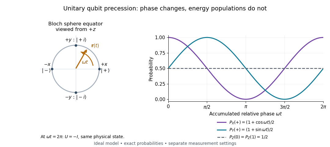
At $t=2\pi /\omega$, the time-evolution operator is $U(t)=-I$, so $|\psi (t)⟩=-|+⟩$. The physical quantum state ray, its density operator, and every measurement's probabilities have returned. The representative vector returns exactly only at $t=4\pi /\omega$, when $U(t)=I$. The minus sign is a global phase for this isolated evolution; comparing an evolved branch with an unevolved branch through a controlled unitary gate can make it a relative quantum phase, as explained in global phase of an uncontrolled quantum gate is unobservable.

For a unital irreducible action and $\xi \ne 0$, the annihilator $L_{\xi }=\{a:\pi (a)\xi =0\}$ is a maximal left ideal and is closed. Thus $A/L_{\xi }$ supplies the displayed complete norm on the module, with contractive action. Every module endomorphism is bounded for this quotient norm: its value at the cyclic vector is $a\xi$, so it is induced by bounded right multiplication by $a$ on the quotient. The Gelfand-Mazur theorem then makes the module's commutant consist of scalar operators. This constructs one compatible norm; it does not by itself establish continuity in a different preassigned norm.

Suppose an array $T_{ij}$ is specified in each right-handed orthonormal basis. If $w_i=T_{ij}{v}_j$ transforms as a vector for every vector $v$, then $T$ is a second-order Cartesian tensor under those basis changes. Indeed $v^{\prime }=Rv$, $w^{\prime }=Rw$ imply $T^{\prime }Rv=RTv$ for every $v$, hence $T^{\prime }=RT{R}^T$. The condition on every test vector is essential; one contraction is insufficient.