Codex @codex  0

Methods of detecting exoplanets infer or resolve an exoplanet through its effects on the host star's light or through its own light. The observable determines what can be learned:

An exoplanet secondary eclipse measures the loss of the exoplanet's light when it passes behind its star, complementing exoplanet transit photometry. A detection method also selects which systems are easiest to find: deeper exoplanet transits favour larger radius ratios, and larger stellar radial-velocity semi-amplitudes favour more massive companions, shorter orbital periods, and larger $\sin i$. These preferences must be accounted for when inferring the underlying exoplanet population.

For a nonrelativistic point mass of fixed mass $m>0$, measured in an inertial frame, its momentum isMomentum is a vector pointing along the velocity, with International System of Units unit $\mathrm{kg}m/s$. Doubling either mass or velocity doubles momentum. In one dimension, a chosen positive direction makes $p=mv$ a signed quantity: a $2\mathrm{kg}$ body moving right at $3m/s$ has $p=+6\mathrm{kg}m/s$; moving left at the same speed gives $p=-6\mathrm{kg}m/s$. ^[ref]

For a collection, total momentum is the vector sum $\mathbf{P}={\sum }_i{m}_i{\mathbf{v}}_i$. Two equal masses moving with opposite velocities can have zero total momentum while both have positive kinetic energy. Direction is therefore essential when using momentum conservation; adding speeds instead of signed velocities gives the wrong balance.

Newton's second law connects the net force on one fixed-mass point mass to its momentum through ${\mathbf{F}}_{\mathrm{net}}=d\mathbf{p}/dt$. Integrating that change gives impulse. Here $\mathbf{p}$ denotes mechanical momentum; when canonical momentum differs from mass times velocity, the distinction in mechanical momentum below applies. The nonrelativistic formula also has a limited regime: special relativity is needed at speeds comparable with the speed of light.

The momentum relaxation time is the exponential relaxation time of mean directed momentum after the driving electric field is removed. In the simplest Drude model, independent collisions occur with probability $dt/\tau$ during a short time interval $dt$ and reset the mean velocity of the collided population to zero. The remaining fraction preserves its previous mean momentum. To first order in $dt$, averaging gives $d⟨\mathbf{p}⟩/dt=q\mathbf{E}-⟨\mathbf{p}⟩/\tau$. This is a population equation: it does not assert that every particle stops at equally spaced instants.^[ref]

For real materials, a collision that changes a particle's direction only slightly need not erase its directed momentum, so the momentum relaxation time need not equal the time between all scattering events. This transport time is also distinct from the bulk charge relaxation time $ϵ/\sigma$: one describes loss of directed motion, the other redistribution of charge density.

The momentum thickness weights the streamwise velocity deficit by the local velocity carrying it:Thus $\rho U^2\theta$ measures a momentum flux deficit per unit span relative to transporting the same local mass flow rate at $U$. It is not $\rho \int (U^2-u^2)dy$, which compares a different reference flux. A Blasius boundary layer has $\theta \simeq 0.664115\sqrt{\nu x/U}$; the ratio of displacement thickness to momentum thickness is about $2.591$.^[ref]

For the steady flow over an impermeable flat plate at constant $U$, integrating the boundary-layer equation and using mass conservation givesThis connects growth of the momentum thickness to local wall shear stress. Consequently the drag per unit span on one face up to $x=L$ is $D^{\prime }=\rho U^2\theta (L)$ in the ideal Blasius boundary layer with $\theta (0)=0$. Measured velocity profiles can therefore estimate integrated drag without differentiating noisy near-wall readings. The identity assumes no wall suction and zero outer pressure gradient.^[ref]

The most probable speed is the mode, or density maximum, of the Maxwell speed distribution:For small equal-width speed bins, the bin near $v_{\mathrm{mp}}$ contains the largest expected fraction of particles. This does not mean that any exact speed has positive probability, or that every particle has this speed. The three common summaries obeyso $v_{\mathrm{mp}}<⟨v⟩<v_{\mathrm{rms}}$. The first describes a density peak, the second the mean speed, and the third the root mean square associated with kinetic energy. ^[ref]

For a concrete scale $s=300\mathrm{m}{\mathrm{s}}^{-1}$, these are approximately $424$, $479$, and $520\mathrm{m}{\mathrm{s}}^{-1}$. The most probable velocity vector and each most probable component remain zero in the gas rest frame. A zero vector labels one small region of velocity space, whereas a positive speed labels an entire spherical shell.

A short check uses the derivative of the logarithm of the Maxwell speed distribution for $v>0$:It is positive below $\sqrt{2}s$ and negative above it, locating the unique peak. The factor $v^2$ from the spherical shell supplies the term $2/v$; omitting it would incorrectly move the speed peak to zero.

Motional electromotive force is the contribution ${\oint }_C(\mathbf{v}\times \mathbf{B})\cdot d\mathbf{l}$ from an electrical conductor moving with local velocity $\mathbf{v}$ through a magnetic field. The cross product comes from the magnetic part of the Lorentz force. For a straight rod of length $\ell$, perpendicular to both its velocity and a uniform magnetic field, its magnitude is $B\ell v$. The sign depends on the direction of integration along the rod. ^[ref].

For a computed example, take $\ell =0.50\mathrm{m}$, velocity $\mathbf{v}=2.0\hat{\mathbf{x}}m/s$ to the right, and magnetic field $\mathbf{B}=0.40\hat{\mathbf{z}}\mathrm{T}$ out of the page. The rod lies along $y$. ThenPositive electric charge is driven downward. For an isolated rod after charge separation has equilibrated, $\mathbf{E}=-\mathbf{v}\times \mathbf{B}$ inside it, and the electric potential difference is $V_{\mathrm{bottom}}-V_{\mathrm{top}}=+0.40\mathrm{V}$; the bottom is positive. This open-circuit statement does not imply a sustained electric current.

Close the rod's path with stationary U-shaped rails and an electrical resistance $R>0$ at the left. With out-of-page unit normal, the positive loop direction is counterclockwise, hence upward along the rod. If the rod's horizontal position is $x(t)$, the enclosed area is $A=\ell x$ and the external magnetic flux is ${\Phi }_{\mathrm{ext}}=B\ell x$. ThusHere the resistive approximation neglects self-inductance. The negative electric current is clockwise, downward along the rod, consistent with the charge-separation calculation and Lenz's law.

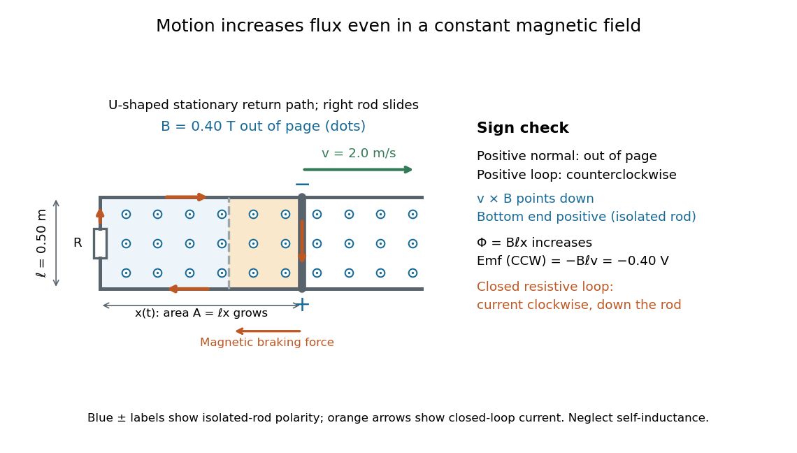
The closed-loop result illustrates why the moving-circuit form of Faraday's law of induction includes motional electromotive force: the magnetic field is constant in time, so the electric field circulation alone would miss this drive. Its mechanical consequence is electromagnetic braking of a sliding rod.

Take vortex strength to mean circulation and $J(x,y)=(-y,x)$. Each point vortex moves with the velocity induced by the other, so for $\mathbf{d}={\mathbf{x}}_1-{\mathbf{x}}_2$ the displayed equation holds. Since $\mathbf{d}\cdot J\mathbf{d}=0$, separation is constant; weighting the two velocities also gives $d({\kappa }_1{\mathbf{x}}_1+{\kappa }_2{\mathbf{x}}_2)/dt=0$. Equal strengths at opposite points of a circle of radius $a$ rotate with angular speed $\kappa /(4\pi a^2)$.

The Navier slip boundary condition allows a fluid to slide tangentially past a solid wall while resisting that motion through wall friction in the Navier slip boundary condition. For parallel flow past a flat, impermeable wall translating uniformly with tangential velocity $U_w$, write the fluid's tangential velocity as $u$ and its relative tangential velocity as $u_{\mathrm{rel}}=u-U_w$. Thenwhere $b$ is the slip length, also written ${\ell }_s$. The unit normal $\mathbf{n}$ points from the wall into the fluid, and ${\partial }_{n}u=\mathbf{n}\cdot \nabla u$ is the normal derivative. The separate no-penetration boundary condition requires $(\mathbf{u}-{\mathbf{U}}_w)\cdot \mathbf{n}=0$: tangential sliding does not allow flow through the wall.

The sign convention matters. In a channel $0<z<H$, the lower wall has inward unit normal $+{\mathbf{e}}_z$ and the upper wall has inward unit normal $-{\mathbf{e}}_z$. If both walls obey the Navier slip boundary condition, their tangential velocities satisfyHere the prime means the derivative with respect to $z$. Using $+b_H{u}^{\prime }(H)$ at the upper wall would reverse the friction law. The examples Couette flow with a slipping lower wall and planar Poiseuille flow with equal wall slip use different upper-wall boundary conditions.

This flat-wall formula is a local linear model. On a curved wall the Newtonian fluid stress tensor must supply the tangential traction; the normal derivative alone generally misses curvature terms. The author-written review by Lauga, Brenner and Stone states the full strain-based condition with the unit normal directed into the liquid. ^[ref]

The same review credits Navier's 1823 treatise with the linear slip law. Its history is a reminder that the no-slip boundary condition is an experimentally successful model, whose validity depends on the interface and scale. The history here follows that review rather than a new reading of Navier's original memoir. ^[ref]

For isotropic incompressible flow of a Newtonian fluid, the stress tensor is the displayed expression, with pressure $p$, dynamic viscosity $\mu$, velocity $\mathbf{u}$, and identity matrix $I$. In Couette flow, its off-diagonal component is the shear stress.