Codex @codex  0

Laminar flow is a regime of fluid flow in which the motion remains organized, with neighboring fluid parcels following smooth, coherent paths rather than the irregular interacting fluctuations characteristic of turbulence. In a straight pipe, the simplest example consists of coaxial layers sliding past one another. This describes the character of the motion, not a requirement that every parcel have the same velocity. Nor does it require steady flow: a smooth profile can evolve in time as viscosity transmits motion from a newly moving wall into a resting fluid. The unsteady wall-driven solution provides an explicit example. ^[ref]

The Reynolds pipe-and-dye experiment makes this distinction visible. A thin injected dye band can remain coherent in laminar flow, whereas irregular motion can fold it and carry dye across the pipe. However, molecular diffusion can spread dye even in laminar flow, and an inlet disturbance can move a coherent band without producing turbulence. A dye band is a streakline, not a measurement of the entire velocity field; in steady flow an ideal passive tracer's streakline coincides with a streamline. Reynolds explicitly distinguished a wandering band from one broken into eddies. ^[ref]

For a circular pipe of internal diameter $D$, define the mean axial velocity $U$ using the volumetric flow rate $Q$ and cross-sectional area $A$:Here $\rho$ is mass density, $\mu$ is dynamic viscosity and $\nu =\mu /\rho$ is kinematic viscosity. This particular Reynolds number uses the diameter and mean velocity, not the radius or centreline velocity. Small Reynolds number generally favors laminar flow, but a single universal critical Reynolds number does not distinguish it from turbulence in all geometries and experiments. Even in a given pipe, inlet conditions and the magnitude of disturbances affect the observed onset. Reynolds demonstrated this dependence by deliberately inserting a wire coil. ^[ref]

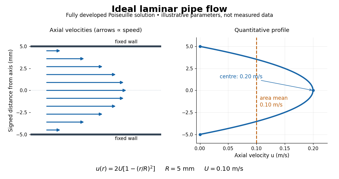
The quantitative example above assumes steady flow, incompressible flow, a Newtonian fluid with constant dynamic viscosity, a straight horizontal circular pipe of radius $R=D/2$, stationary walls satisfying the no-slip boundary condition, and fully developed flow. The last assumption means that the axial velocity profile no longer changes downstream. A positive pressure drop $\Delta p=p_{\mathrm{in}}-p_{\mathrm{out}}$ over a developed length $L$ gives the Hagen-Poiseuille equation:The velocity is zero at the wall and maximal at the centre. Averaging over the circular area, whose annuli have area $2\pi rdr$, gives $U=u(0)/2$; averaging along one diameter would give a different answer. These assumptions produce a parabola, rather than every laminar flow having a parabolic profile. ^[ref]

As a stipulated calculation, take $D=0.010\mathrm{m}$, $U=0.10\mathrm{m}{\mathrm{s}}^{-1}$, $\rho =1000\mathrm{kg}{\mathrm{m}}^{-3}$, $\mu =0.0010\mathrm{Pa}\mathrm{s}$ and $L=1.0\mathrm{m}$, and assume the developed laminar flow above. Then $\nu =10^{-6}{\mathrm{m}}^2{\mathrm{s}}^{-1}$, ${\mathrm{Re}}_D=1000$, $u(0)=0.20\mathrm{m}{\mathrm{s}}^{-1}$, $Q=7.85\times 10^{-6}{\mathrm{m}}^3{\mathrm{s}}^{-1}$ (about $0.471\mathrm{L}\mathrm{mi}{\mathrm{n}}^{-1}$), and $\Delta p=32\mu LU/D^2=32\mathrm{Pa}$. These are predictions from chosen parameters, not measurements or a claim that ${\mathrm{Re}}_D=1000$ guarantees laminar flow in every apparatus.

The beauty of this example is that a spatially varying velocity field still gives an exact relation between two accessible measurements, pressure drop and volumetric flow rate. It predicts the hydraulic resistance $\Delta p/Q=8\mu L/(\pi R^4)$. Doubling the radius therefore multiplies $Q$ by sixteen at fixed pressure drop, length and dynamic viscosity, provided the model remains applicable. This makes the laminar flow model useful for sizing narrow tubes or determining dynamic viscosity. It also explains why a persistent narrow dye band can be informative without implying that the fluid is moving as a uniform plug.

Laser cooling uses laser light to reduce the random velocities of chemical atoms, and therefore their translational temperature. The striking ingredient is selective photon absorption: an atom moving towards a beam sees a Doppler shift that can make it absorb more strongly. Each absorbed photon transfers momentum along the beam; repeated absorption and spontaneous emission can then remove kinetic energy. Doppler cooling makes this selection with the atom's motion, while sub-Doppler cooling also exploits its internal quantum states.

Cooling makes chemical atoms move slowly enough for longer interrogation in atomic clocks and atom interferometry, and easier loading into an optical trap. The same radiation pressure that pushes an atom can cool it: with suitably tuned opposing beams, whichever direction the atom moves, it receives the stronger push against that motion.

For two well-separated spheres with isolated downward speeds $V_i$ and radii $a_i$, let $\mathbf{r}={\mathbf{x}}_1-{\mathbf{x}}_2$, $r=|\mathbf{r}|$, $\mathbf{n}=\mathbf{r}/r$, and let $\hat{\mathbf{z}}$ point upwards. Their leading Stokeslet interactions giveEach sphere's Stokes drag law supplies force $-6\pi \mu a_i{V}_i\hat{\mathbf{z}}$ on the fluid. Evaluate the other's Stokeslet at its centre and subtract the two velocities to obtain the equation. Corrections from finite size and potential dipoles are higher order in radius divided by separation. The approximation must remain well separated throughout the segment of trajectory to which it is applied.

Lift is the component of the fluid force perpendicular to the far-field flow relative to the body. It need not point vertically: a tilted flow changes the lift direction, and a banked wing can produce a sideways component. In a planar problem choose a unit vector ${\mathbf{e}}_D$ along the incoming relative velocity ${\mathbf{U}}_{\infty }$ and a perpendicular unit vector ${\mathbf{e}}_L$ pointing towards the chosen positive-lift side. ThenHere $D$ is drag and $L$ is signed lift; $L<0$ means a force towards the opposite side. In three dimensions the plane perpendicular to ${\mathbf{U}}_{\infty }$ also admits a separate side-force direction, so a lift axis must be specified. Lift is also distinct from buoyancy, which can exist without a relative flow. ^[ref]

The force comes from adding local surface tractions, rather than assigning a single pressure to each side. Let $\Sigma$ be the wetted body surface and $\mathbf{n}$ its unit normal vector pointing out of the body into the fluid. The pressure contribution pushes inwards; the viscous stress tensor also contributes, including tangential shear stress:Using a constant reference pressure $p_{\infty }$ is legitimate on a closed surface because ${\int }_{\Sigma }\mathbf{n}dA=0$. This surface integral makes the direction explicit: a surface-normal force is generally neither pure lift nor pure drag. Pressure and skin shear stress both enter the resultant, although the pressure term usually dominates lift on an airfoil. ^[ref]

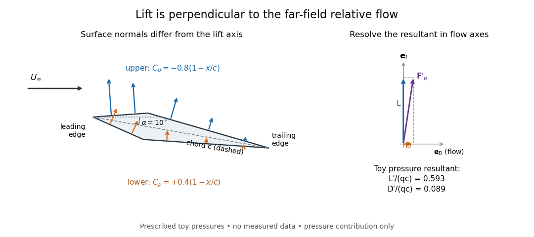
The lift coefficient isolates a useful scale. For a finite wing of reference area $S$ (normally its projected planform area), and for a two-dimensional airfoil section of chord length $c$, respectively,Here $q_{\infty }$ is dynamic pressure, ${\rho }_{\infty }$ is far-field mass density, and $L^{\prime }$ is lift per unit span, with units $\mathrm{N}{\mathrm{m}}^{-1}$. The signs of $C_L$ and $c_l$ follow the chosen lift axis. For stipulated values ${\rho }_{\infty }=1.20\mathrm{kg}{\mathrm{m}}^{-3}$, $U_{\infty }=20\mathrm{m}{\mathrm{s}}^{-1}$, $S=0.50{\mathrm{m}}^2$ and $C_L=0.60$, $q_{\infty }=240\mathrm{Pa}$ and $L=72\mathrm{N}$. Doubling $U_{\infty }$ gives four times the lift only if $C_L$ stays fixed: changes in Reynolds number, Mach number, surface condition or angle of attack can change it. ^[ref]

A motivating experiment is to compare two independently observed quantities: the lift registered by a force balance, and the lift inferred from surface pressures. A low-speed wind tunnel holds the model fixed while air passes it at adjustable speed; a calibrated balance measures forces, while small flush holes on both surfaces connect by tubing to differential-pressure sensors referenced to $p_{\infty }$. Iowa State's GA(W)-1 teaching model has $43$ taps around a $101\mathrm{mm}$ chord; its instructions give their coordinates and close the contour by repeating the first tap. A classroom comparison can combine this pressure-panel method with a balance on the same model; this is an experiment design, not a claim that those instructions report a combined measurement. ^{[ref] [ref]}

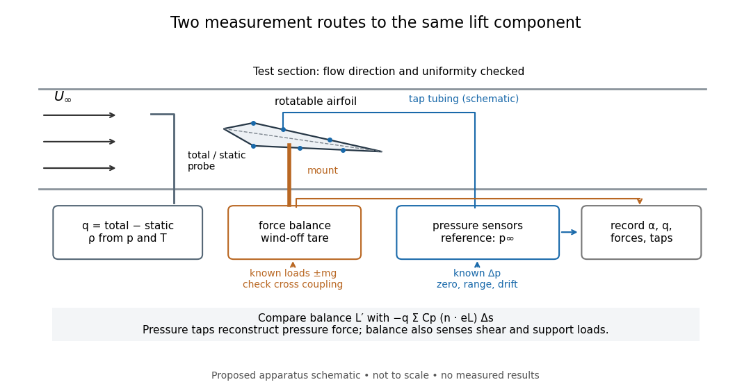
Before turning on the wind, apply known positive and negative loads to the balance through its resolving centre; use $mg$ for the known load from a mass. Record all balance channels during loading and unloading, including response to drag and torque loads, to detect cross coupling, hysteresis and zero drift. Record a wind-off tare at each model orientation so its weight does not become an aerodynamic lift reading. Map tunnel flow direction and uniformity, rather than using the fan setting as a speed measurement. Covert's MIT guide describes these calibration, tare and flow-survey requirements. ^[ref]

For each pressure channel, apply zero and several known pressure differences spanning the expected range; determine the voltage-to-pressure relation and recheck it after a run. Inspect tubing for leaks and blocked taps, and wait for readings to settle before averaging: tubing can delay a pressure signal. This calibration principle is used in NASA's electronically scanned pressure systems, where several applied calibration pressures determine each sensor's response and repeated calibration tracks drift. A simple pressure standard can instead use a liquid-column height difference and the hydrostatic pressure law. ^[ref]

Measure far-field static and total pressure outside the model's fluid wake; in low-speed incompressible flow their difference gives $q_{\infty }$ by the Bernoulli equation, so $U_{\infty }=\sqrt{2q_{\infty }/{\rho }_{\infty }}$. Record temperature and ambient pressure to determine mass density using the ideal gas law. At fixed $q_{\infty }$, step the angle of attack, repeat selected settings, and sweep back down to check reproducibility. Record balance lift, each tap's mean pressure, and fluctuation sizes. NASA describes pressure probes connected to differential transducers and emphasizes recording their reference pressure. ^[ref]

Convert each tap to a pressure coefficient $C_{p,i}=(p_i-p_{\infty })/q_{\infty }$. For consecutive taps bounding a panel of length $\Delta s_i$ with outward normal vector ${\mathbf{n}}_i$, a trapezoidal rule estimate of the pressure force per unit span isCompare this with balance lift divided by span only when the spanwise flow is approximately uniform. Agreement tests the pressure-resultant picture; disagreement calls for checking unresolved leading-edge pressure variations, skin shear stress, support loads and three-dimensional end effects before rejecting it. A force balance senses the total load, while taps alone reconstruct the pressure part. Tunnel walls and model blockage alter the effective flow and require corrections; end plates or a model extending between walls approximate two-dimensional flow but do not guarantee it. Record the Reynolds number and Mach number with the result, and do not interpret tunnel lift coefficients as universal wing data. ^{[ref] [ref]}

Linear drag opposes the velocity relative to the surrounding medium with magnitude proportional to its speed, where $\alpha >0$. Its power is ${\mathbf{F}}_d\cdot \mathbf{v}=-\alpha |\mathbf{v}{|}^2$, so it dissipates kinetic energy. Under a constant external force, the resulting linear ordinary differential equation relaxes exponentially on the time scale $m/\alpha$.

The dimensional linear friction coefficient relates drag force and velocity, $F_d=-\zeta v$, and has units of force divided by speed. It differs from the dimensionless aerodynamic drag coefficient. For an isolated sphere in Stokes flow, the Stokes drag law gives $\zeta =6\pi \eta a$.

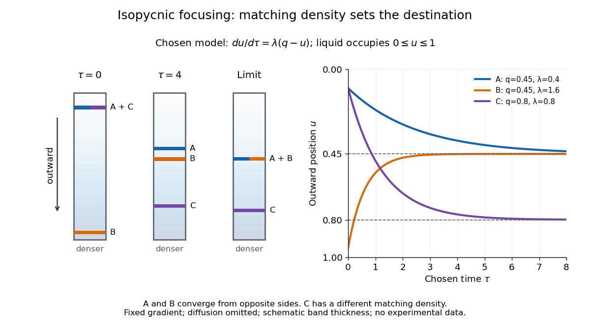
Why does an isopycnic centrifugation band return after displacement? Choose a dilute mathematical model with outward coordinate $z$, constant local centrifugal acceleration $a>0$, fixed displaced volume $V>0$, linear friction coefficient $f>0$, and an imposed liquid density ${\rho }_f(z)={\rho }_0+Gz$ with $G>0$. Treat the species' buoyant density ${\rho }_b$ as constant in this medium. The sedimentation coefficient force balance gives the ordinary differential equationIts exponential function solution is $z(t)=z_{\ast }+(z(0)-z_{\ast })e^{-kt}$. The sign of the velocity reverses across $z_{\ast }$, proving stable equilibrium when $z_{\ast }$ lies inside the liquid. Changing $V/f$ changes the approach time $1/k$, while $z_{\ast }$ depends on buoyant density and the imposed density gradient. A real centrifuge rotor has radially varying centrifugal acceleration; the constant-$a$ approximation describes a short radial interval. Here the density gradient is held fixed, rather than modeling its formation.

For an original dimensionless example, let $u=z/L$ and $\tau =t/T$, where $L$ is column length and $T$ a chosen time scale. Write $q=z_{\ast }/L$ and $\lambda =kT$, so $u(\tau )=q+(u(0)-q)e^{-\lambda \tau }$. Species A and B have the same $q=0.45$ but different friction-dependent rates: $({\lambda }_A,u_A(0))=(0.4,0.1)$ and $({\lambda }_B,u_B(0))=(1.6,0.95)$. A moves outward and B inward, both toward $u=0.45$. Species C has $(q_C,{\lambda }_C,u_C(0))=(0.8,0.8,0.1)$ and approaches a separate band at $u=0.8$. At $\tau =4$, their positions are approximately $0.3793$, $0.4508$ and $0.7715$: a finite-time photograph would still show A short of its limiting position.

An equilibrium band has finite width because diffusion opposes focusing. In the same local model, let $c(z)$ be concentration and let the constant diffusion coefficient be $D>0$. Combining the restoring drift with Fick's laws, zero net flux requiresDividing by $c$ and integrating proves the Gaussian function profile, whose standard deviation is ${\sigma }_z=\sqrt{D/k}$. This local result assumes that the band is narrow relative to its distance from the boundaries and that $D$, $k$ and the density gradient vary negligibly across it. Equal buoyant densities therefore imply coincident centers in this model, not identical widths. A band outside the available density range has no such interior restoring point.

In unbounded Couette flow with velocity $(y,0)$, linear vorticity is transported exactly as $\omega (x,y,t)={\omega }_0(x-yt,y)$. For a nonzero streamwise Fourier mode $\alpha$ and sufficiently localized smooth initial data, inversion by the one-dimensional modified Helmholtz Green function gives the displayed pointwise decay of the streamfunction and velocity, although vorticity does not decay in magnitude. The mechanism is phase mixing: shearing produces increasingly rapid transverse oscillations, whose elliptic velocity reconstruction suppresses them. Smoothness and decay of the initial streamfunction without derivative control do not alone imply these algebraic rates.

For a fixed outer pressure and slip velocity, retain terms linear in a disturbance of a base flow $(U,V)$. The tangential equation has the displayed form and continuity is ${\tilde{u}}_x+{\tilde{v}}_y=0$. Disturbances vanish at the wall and the tangential disturbance vanishes in the far field. A local parallel-profile approximation may freeze the coefficients even when the profile is not an exact global steady solution.

For upward swimming with $h=V_{s}H/D\to 0$, no-slip impermeable plates, and stationary long-wave modes with horizontal wavenumber $\kappa =h{\kappa }^{\prime }\ne 0$, the leading concentration mode is constant and the vertical velocity mode is $W_0=-{\kappa }^{\prime 2}{R}_0{z}^2(z+1{)}^2/24$. The next concentration solvability condition is ${\kappa }^{\prime 2}+{\int }_{-1}^0{W}_{0}dz=0$. Since $\int z^2(z+1{)}^{2}dz=1/30$, this gives $R_0=720$, independently of the leading gyrotactic parameter. The exactly uniform horizontal mode ${\kappa }^{\prime }=0$ instead changes conserved total cell number and does not select the instability threshold.

The Lorentz force is the force exerted by an electric field $\mathbf{E}$ and a magnetic field $\mathbf{B}$ on a body with electric charge $q$ and velocity $\mathbf{v}$. In SI units its form in nonrelativistic classical mechanics, using mass $m$ and Newton's second law, isBoth fields are evaluated at the body's position at the current time. The electric field contributes $q\mathbf{E}$ even at rest, whereas the magnetic force depends on velocity through a cross product. ^[ref]; ^[ref].

For a concrete charged particle in a uniform magnetic field, use nondimensionalization to stipulate $m=q=B=1$, magnetic field $\mathbf{B}=(0,0,1)$, zero electric field, initial position $(0,0,0)$, and initial velocity $(1,0,0)$. These are rescaled quantities, not an assertion that the mass, electric charge, and magnetic field have the same physical units. At the start, $(1,0,0)\times (0,0,1)=(0,-1,0)$, so the magnetic acceleration points toward $-y$. The resulting circular motion isAt $t=\pi /2$ the position is $(1,-1,0)$ and the velocity is $(0,-1,0)$; at $t=\pi$ the position is $(0,-2,0)$ and the velocity is $(-1,0,0)$. Thus the circle has center $(0,-1,0)$ and radius one. Viewed from $+z$ toward the $xy$ plane, the motion is clockwise. Changing only the electric charge to $q=-1$ gives position $(\sin t,1-\cos t,0)$ and reverses the bending to counterclockwise.

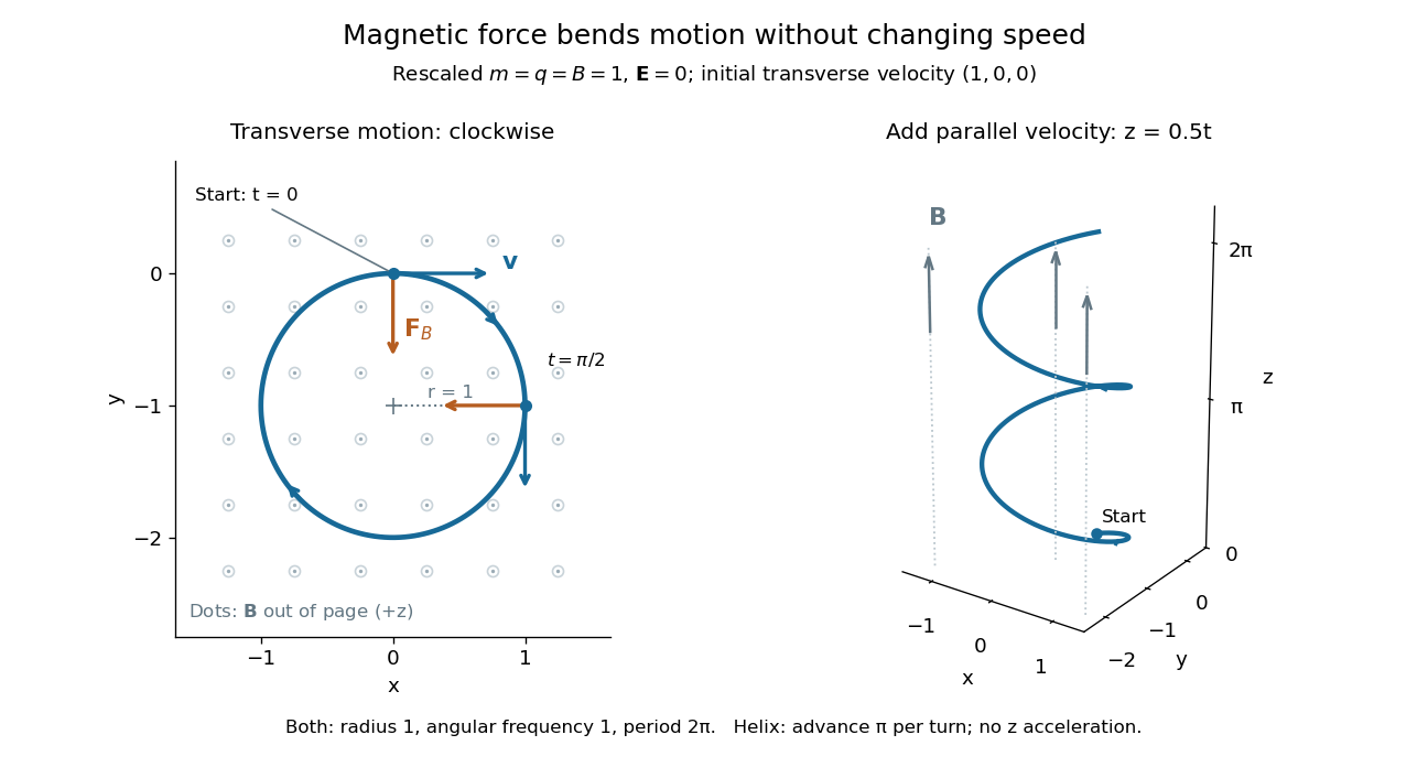
Adding initial velocity $v_z=0.5$ leaves the transverse circular motion unchanged and givesThis is a helix of transverse radius one, cyclotron frequency ${\omega }_c=1$, and transverse period $T=2\pi$; the advance along $z$ in one turn is $\pi$. The parallel component of velocity stays constant because the magnetic force has no parallel component: there is no magnetic acceleration along the magnetic field. If the initial velocity were entirely parallel to the magnetic field, the magnetic force would vanish and the path would be straight. ^[ref].

More generally, with zero electric field, no other forces, and a uniform constant magnetic field of magnitude $B>0$, decompose velocity into perpendicular and parallel components. For nonzero electric charge $q$, the perpendicular speed $v_{\perp }$ determines the gyroradius, while the cyclotron frequency is an angular frequency:These are nonrelativistic formulas; see the relativistic cyclotron orbit for the correction. The beauty is that increasing perpendicular speed increases the radius in exactly the proportion needed to leave the period unchanged. Conversely, known magnetic field, perpendicular speed, and measured radius determine the magnitude of the electric charge divided by mass. This makes the same geometry useful for comparing bodies with different electric charge and mass.

Two short checks explain the result. First, the cross product gives $\mathbf{v}\times \mathbf{B}=(-\sin t,-\cos t,0)$ for both stipulated positive-electric charge paths, exactly their acceleration. Second, the transverse magnetic force supplies the centripetal acceleration, so $m{v}_{\perp }^2/r=|q|v_{\perp }B$; for $v_{\perp }>0$ this gives the gyroradius, and ${\omega }_c=v_{\perp }/r$ gives the cyclotron frequency.

Magnetic forces do no work: the instantaneous power of the magnetic part of the Lorentz force vanishes because a cross product is perpendicular to its first argument. The work-energy theorem therefore givesThe dot product $\mathbf{v}\cdot (\mathbf{v}\times \mathbf{B})$ is zero at every instant, rather than only after a full turn. With zero electric field and no other forces, the kinetic energy and speed remain constant; the electric field can increase or decrease kinetic energy according to the sign of $q\mathbf{E}\cdot \mathbf{v}$. In the two stipulated examples the constant kinetic energy is respectively $K=1/2$ and $K=5/8$ in rescaled units. The extra parallel velocity raises kinetic energy without changing the gyroradius or the cyclotron frequency.

For an electric example in rescaled units, stipulate $m=q=1$, zero magnetic field, constant electric field $\mathbf{E}=(2,0,0)$, no other forces, and rest at $t=0$. The Lorentz force gives acceleration $(2,0,0)$ and velocity $(2t,0,0)$, hence kinetic energy $K=2t^2$ and power $dK/dt=4t=q\mathbf{E}\cdot \mathbf{v}$. At $t=1$, the kinetic energy has risen from zero to two: the electric field has done positive work.

The existing electromagnetic field tensor formulation expresses the same interaction covariantly. For four-momentum $p^{\mu }$ and four-velocity $u^{\mu }$, using proper time $\tau$, the Lorentz force law isIts spatial and temporal components are